Graphs - UCF CAP-6318

Computational Analysis of Social Complexity
Fall 2025, Spencer Lyon

Prerequisites

Julia setup
Julia basics
Julia types and methods

Outcomes

Understand key components of networks/graphs
Use the Graphs.jl package for working with graphs in Julia
Implement the breadth-first search algorithm

References

Easley and Kleinberg chapter 2

Introduction¶

Why Study Graphs?¶

Economic, cultural, political, and social interactions are influenced by structure of relationships
- Transmission of viruses
- International trade, supply chains, marketplaces
- Spread of information, diffusion of innovation
- Political persuasion, localized voting patterns
- Human behaviors influenced by network of friends (sports, clothes, music)
Behaviors can be effected by social networks
- “Influencers”
- Circles of followers can create echo chambers

Edges and Nodes¶

A graph specifies relationships between a collection of items
Each item is called a node
A relationship between nodes is represented by an edge
Visually, graphs might look like this:

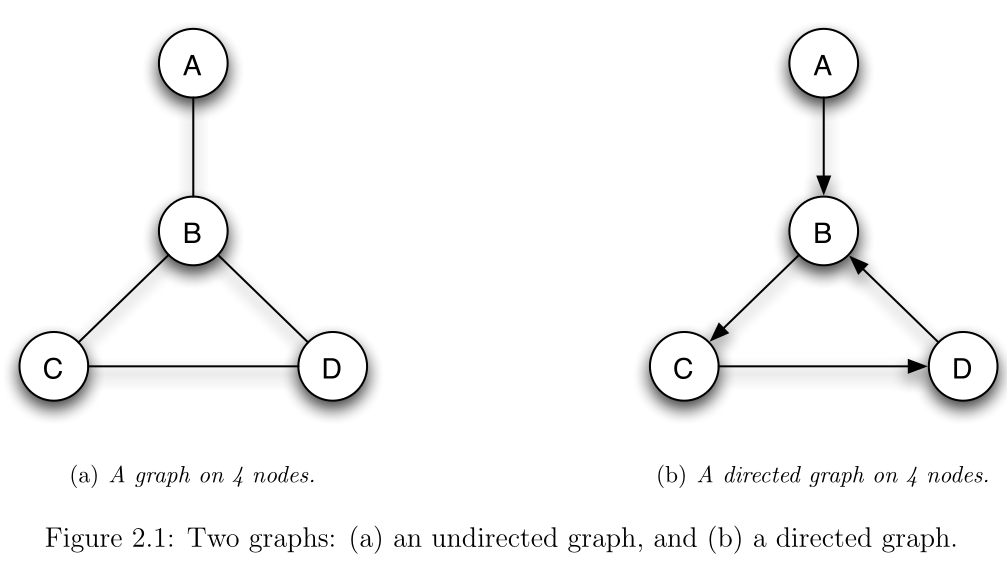
Here the nodes are A, B, C, D
The edges connect nodes A-B, B-C, B-D, C-D

Adjacency Matrix¶

How might we represent the graph above numerically?
One very common approach is to use a matrix of 0’s and 1’s called an adjancency matrix
Suppose we have a graph of $N$ nodes
- Without loss of generality, we’ll represent them as integers 1:N
Let $A \in \{0,1\}^{N \times N}$ be our adjacency matrix
Element $A_{ij}$ will be zero unless there is an edge between nodes $i$ and $j$ (diagonal is left as 0)
In our above we had
- Nodes A, B, C, D (or 1, 2, 3, 4 respectively)
- Edges connecting nodes 1-2, 2-3, 2-4, 3-4
The adjacency matrix for this example is
$A = \begin{bmatrix} 0 & 1 & 0 & 0 \\ 1 & 0 & 1 & 1 \\ 0 & 1 & 0 & 1 \\ 0 & 1 & 1 & 0 \end{bmatrix}$
(1)

Graphs in Julia¶

In Julia there are a few ways we could represent our example graph above
We could start with the adjacency matrix concept as follows

4×4 Matrix{Int64}:
 0  1  0  0
 1  0  1  1
 0  1  0  1
 0  1  1  0

Working with Adjacency Matrices¶

An adjacency matrix gives us a lot of information about the structure of the graph
We could compute all of the following
- Total number of nodes: number of rows or columns of $A$
- Total number of edges: $\sum_{ij} A_{ij}$
- Node with most edges: $\text{argmax}_{i} \sum_{j} A_{i,j}$
- Average number of edges per node: $\frac{2}{N} \cdot \sum_{i,j>i} A_{i,j}$

Exercise: Adjacency Matrix¶

In the cell below we have defined an adjacency matrix called A_ex1
Using A_ex1 answer the following questions:
- How many nodes are in the graph?
- How many edges?
- Node with most edges (hint, use the dims argument to sum and then the argmax function)
- Average number of edges per node
- Number of connections for node 7: $\sum_j A_{j7}$

import Random
Random.seed!(42)

A_ex1 = zeros(Int, 30, 30)

for i in 1:30
    for j in (i+1):30
        if rand() < 0.2
            A_ex1[i, j] = 1
            A_ex1[j, i] = 1
        end
    end
end

# Your code here

ex1_total_nodes = missing
ex1_total_edges = missing
ex1_node_most_edges = missing
ex1_average_edges_per_node = missing
ex1_connections_node_7 = missing

missing

Graphs.jl¶

There are many smart graph theory experts in the Juila community
They have built a package called Graphs for working with graphs (as well as ancillary pacakges for extra features)
We can build a Graphs.Graph object directly from our adjacency matrix

using Graphs

G1 = Graph(A)

{4, 4} undirected simple Int64 graph

collect(edges(G1))  # collect turns an `iterator` into an array

4-element Vector{Graphs.SimpleGraphs.SimpleEdge{Int64}}:
 Edge 1 => 2
 Edge 2 => 3
 Edge 2 => 4
 Edge 3 => 4

collect(vertices(G1))  # Graphs refers to nodes as `vertices`

4-element Vector{Int64}:
 1
 2
 3
 4

Visualizing Graphs¶

We can use the GraphPlot package to visualize our graph
Note that the actual placement of the nodes is randomly generated and then tweaked to clearly show all nodes and edges
The important thing is not the placement of nodes, but rather their relative structure

using GraphPlot  # load GraphPlot package

gplot(G1)

Size considerations¶

Using Array{Int64,2} to store an adjacency matrix turns out to be a rather costly way to store a graph
In the original example graph we had 4 nodes and 4 edges
To store this we needed to have a 4x4 matrix of 64 bit integers
- This is only (Int(16 * 64 / 8) == 128) bytes in our exapmle,
- But consider a graph of websites and links between them -- that graph would have millions of nodes and edges...
There are a few approaches to reducing this storage cost:
- Only store the upper triangle of the matrix
- Use Array{Bool,2} instead of Array{Int64,2} to store adjacency matrix ( each element only sizeof(Bool) == 1 bit!)
- Use a SparseMatrix
- Store as a Vector{Vector{Int}}

# Vector{Vector{Int}}
A2 = [[2], [1, 3, 4], [2, 4], [2, 3]]

4-element Vector{Vector{Int64}}:
 [2]
 [1, 3, 4]
 [2, 4]
 [2, 3]

G1.fadjlist

4-element Vector{Vector{Int64}}:
 [2]
 [1, 3, 4]
 [2, 4]
 [2, 3]

Graph Theory Concepts¶

Let’s explore some concepts often used in analysis of graphs

Paths¶

When studying graphs it is often natural to ask about how things travel or flow across the graph
For example, how information spreads amongst a group of friends, how data travels the internet, how diseases are transmitted from one person to another, and how people navigate a metro subway system
In each of these cases, the flow of things goes from node to node across edges
A flow from one any node to another node is called a path

Degree¶

The degree of a node is the number of edges connected to it
In our example graph G1, node B has degree 3 (connected to A, C, and D)
Node A has degree 1 (only connected to B)
Degree is a fundamental measure of node importance in a network
- High-degree nodes are often called “hubs”
- In social networks, these might be influential people or “connectors”
We can compute degree directly from the adjacency matrix
- Degree of node $i$ is $\sum_j A_{ij}$
Graphs.jl provides the degree function

degree(G1)

4-element Vector{Int64}:
 1
 3
 2
 2

degree(arpa, node_ints["MIT"])

UndefVarError: `arpa` not defined in `Main`

Suggestion: check for spelling errors or missing imports.



Stacktrace:

 [1] top-level scope

   @ ~/Teaching/UCF/CAP-6318/book-myst/week03/jl_notebook_cell_df34fa98e69747e1a8f8a730347b8e2f_Y164sZmlsZQ==.jl:1

The degree distribution of a network tells us a lot about its structure
Many real-world networks have a few high-degree hubs and many low-degree nodes
- Social networks: celebrities with millions of followers
- Internet: major websites with many incoming links
- Transportation: hub airports like Atlanta or Chicago

Arpanet Example¶

Consider the following Graph of the first iteration of the internet

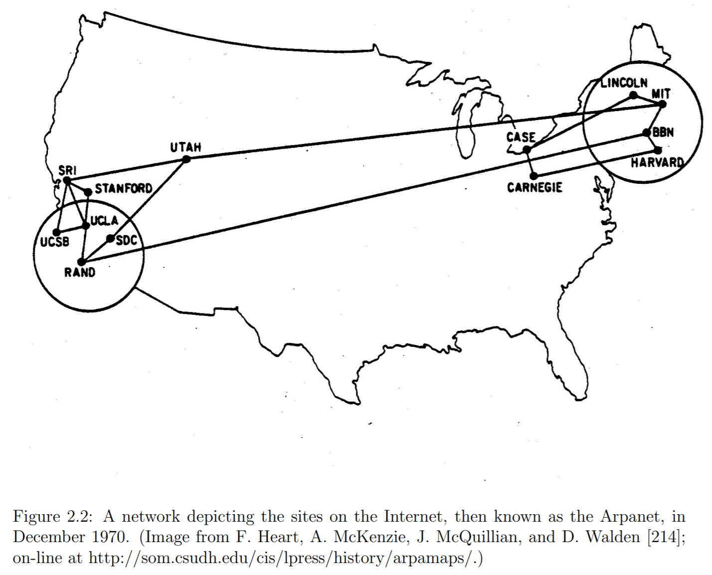
There are many possible paths through this network
Consider a path from UCSB to MIT: UCSB-UCLA-RAND-BBN-MIT
Another possible path from UCSB to MIT is UCSB-SRI-UTAH-MIT

Graphs.jl Arpanet¶

Let’s define the Arpanet using Graphs as it will be helpful throughout this lecture

nodes = [
		"UCSB" => ["SRI", "UCLA"],
		"SRI" => ["UCSB", "UCLA", "STAN", "UTAH"],
		"UCLA" => ["SRI", "UCSB", "STAN", "RAND"],
		"STAN" => ["SRI", "UCLA"],
		"UTAH" => ["SRI", "SDC", "MIT"],
		"SDC" => ["UTAH", "RAND"],
		"RAND" => ["UCLA", "SDC", "BBN"],
		"MIT" => ["UTAH", "BBN", "LINC"],
		"BBN" => ["MIT", "RAND", "HARV"],
		"LINC" => ["MIT", "CASE"],
		"CASE" => ["LINC", "CARN"],
		"CARN" => ["CASE", "HARV"],
		"HARV" => ["CARN", "BBN"]
	]
node_ints = Dict(zip(first.(nodes), 1:length(nodes)))
arpa = SimpleGraph(length(nodes))
for (node, edges) in nodes
    for e in edges
        add_edge!(arpa, node_ints[node], node_ints[e])
    end
end

# save graph for loading in future
savegraph("arpanet.lg", arpa)

1

arpa

{13, 17} undirected simple Int64 graph

gplot(arpa, nodelabel=first.(nodes))

Cycles¶

An important concept when analyzing graphs is the concept of a cycle
A cycle is a path that starts and ends at the same node
For the ARPA net, an example cycle is LINC-CASE-CARN-HARV-BBN-MIT-LINC
Question... what is the shortest possible cycle in a graph (including all endpoints)?
Cycles appear frequently in real-world networks
- Friendship networks: if A is friends with B, and B with C, often A and C become friends
- Transportation networks: cyclical routes allow for redundancy and flexibility
- Supply chains: cyclical dependencies can create both resilience and vulnerabilities

Trees¶

A tree is a connected graph with no cycles
Trees have exactly N-1 edges for N nodes (the minimum to stay connected)
Adding any edge to a tree creates a cycle
Removing any edge from a tree disconnects it
Trees appear frequently in hierarchical structures
- Organizational charts: CEO at root, departments as branches
- Family trees: ancestors and descendants
- Decision trees: choices branching from initial state
- File systems: directories and subdirectories
The breadth-first search we’ll see later naturally creates a tree from any graph

# Example: create a simple tree
tree = SimpleGraph(5)
add_edge!(tree, 1, 2)
add_edge!(tree, 1, 3)
add_edge!(tree, 2, 4)
add_edge!(tree, 2, 5)
gplot(tree, nodelabel=1:5)

is_tree(tree)  # Graphs.jl can check if a graph is a tree

true

is_tree(G1)  # Our original graph has a cycle, so it's not a tree

false

Connectedness¶

A graph is connected if there exists a path between every pair of nodes
In other words, you can travel from any node to any other node by following edges
The ARPA network was designed to be connected -- ensuring communication between all sites
We can check if a graph is connected using Graphs.jl

is_connected(arpa)

true

It is natural to believe that many real-world networks are connected
- Transportation: you can get to any station
- Internet: you can visit any website
But it is entirely possible to have a non-connected graph
- Social networks (nodes: people, edges: friendships) of college students who different countries
- Suppliers for a textile company vs a microchip manufacturer

Distance¶

We can extend concept of paths between nodes, to include a notion of distance
The length of a path is the number of steps it takes from beginning to end
- MIT-BBN-RAND-UCLA has length 3 (starting from MIT take three steps before ending at UCLA)
The distance between two nodes, is the length of the shortest path between those nodes
Graphs can compute distances using the gdistances function
Below we compute the distance between UCLA and all nodes

Dict(zip(first.(nodes), gdistances(arpa, node_ints["UCLA"])))

Dict{String, Int64} with 13 entries:
  "HARV" => 3
  "UTAH" => 2
  "UCSB" => 1
  "LINC" => 4
  "RAND" => 1
  "MIT"  => 3
  "CASE" => 5
  "SRI"  => 1
  "STAN" => 1
  "UCLA" => 0
  "SDC"  => 2
  "CARN" => 4
  "BBN"  => 2

Breadth-First Search¶

If asked, how would you go about computing the distance between the HARV node and all other nodes?
One iterative approach might be:
- Start with HARV: note it is distance zero to HARV
- Move on to all nodes directly connected to HARV: these are distance 1
- Then move to all nodes connected to nodes that are distance 1 from HARV (excluding any you may have already found): declare these to be at distance 2 from HARV
- Continue traversing edges until you have visited all nodes
This algorihtm is called breadth-first search

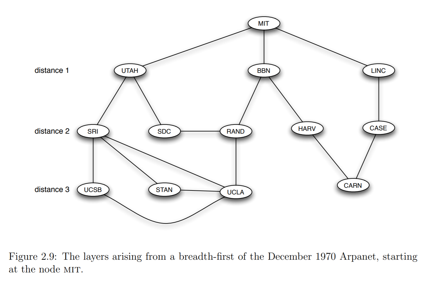
Example: Breadth-First Search from MIT¶

The image below shows how breadth-first search would proceed for the MIT node

Exercise (difficult!): BFS¶

Now it is time for you to try this out!
Our goal is to use breadth-first search to compute the distance betwen a given node and all other nodes
The return value you end up with should be an Vector{Vector{Int}}, where element i of this vector contains all node labels at distance i from the starting node
Fill in the logic for the breadth_first_distances function below

function breadth_first_distances(g, start::Int)
	out = Vector{Int}[]
	# use push!(out, new_nodes) to add to out
	distance = 0

	# TODO: your code here...

	# return out
	out
end

breadth_first_distances (generic function with 1 method)

# Test code

function test_bfd_methods(val, want)
    if length(val) == 0
        error("Make sure to `push!` on to `out` in your function")
    elseif length(val) != maximum(gdistances(arpa, node_ints["HARV"]))
        error("`out` has incorrect number of elements")
    elseif length.(val) != length.(want)
        error("Right number of elements, but not right number in each subvector")
    elseif all(map(x12 -> all(sort(x12[1]) .== sort(x12[2])), zip(val, want)))
        println("correct!")
    end
end

function run_tests()
    val = breadth_first_distances(arpa, node_ints["HARV"])
    want = [[9, 12], [7, 8, 11], [3, 6, 5, 10], [1, 2, 4]]
    test_bfd_methods(val, want)
end

run_tests (generic function with 1 method)

# uncomment the code below and run when you are ready to test your code
# run_tests()

BFS with Graphs¶

The Graphs library contains routines implementing breadth-first search
The main function is called bfs_tree

bfs_carn = bfs_tree(arpa, node_ints["CARN"])

{13, 12} directed simple Int64 graph

Notice that the printout says we have a graph with 13 nodes, 12 edges and it is a directed graph
Thus far, all graphs we have considered have been undirected
- We have only been concerned about if a connection (edge) exists between nodes
A directed graph extends the notion of connecting nodes with a direction
- We can now say that things flow across edges from one node to another -- always in the same direction
Why would the breadth-first search routine return a directed graph instead of the undirected type we started with?
Let’s visualize it and see if we can understand why

gplot(bfs_carn, nodelabel=first.(nodes))

Notice that arrows only flow out of CARN
They also always flow away from CARN
The use of directed edges allows Graphs to represent the shortest path from CARN to any other node
- For example STAN: CARN -> HARV -> BBN -> RAND -> UCLA -> STAN

Exercise: Explore DiGraph¶

The bfs_carn object has type $(Markdown.Code(string(typeof(bfs_carn))))
Let’s view the names of its properties (properties)

propertynames(bfs_carn)

(:ne, :fadjlist, :badjlist)

bfs_carn.fadjlist

13-element Vector{Vector{Int64}}:
 []
 []
 [1, 2, 4]
 []
 []
 []
 [3, 6]
 [5]
 [7, 8]
 []
 [10]
 [11, 13]
 [9]

The fadjlist (forward adjacency list) property is a Vector{Vector{Int64}}
fadjlist has one element per node (call index into outer Vector i for node i)
Each element is itself a vector containing node indices for all nodes j for which there is an edge flowing from i to j
Below we have set up a new method (see below) for the breadth_first_distances function that takes a DiGraph as an argument
Your task is to implement the the method so that it has the same return value as the previous method from above

function breadth_first_distances(g::SimpleDiGraph, start::Int)
	out = Vector{Int}[]
	# use push!(out, new_nodes) to add to out
	distance = 0

	# TODO: your code here...

	# return out
	out
end

breadth_first_distances (generic function with 2 methods)

# test code
function test_digraph_ex()
	val = breadth_first_distances(
		bfs_tree(arpa, node_ints["HARV"]),
		node_ints["HARV"]
	)
	want = [[9, 12], [7, 8, 11], [3, 6, 5, 10], [1, 2, 4]]
	test_bfd_methods(val, want)
end

test_digraph_ex (generic function with 1 method)

# uncomment the code below when you are ready to test your code!
# test_digraph_ex()

Components¶

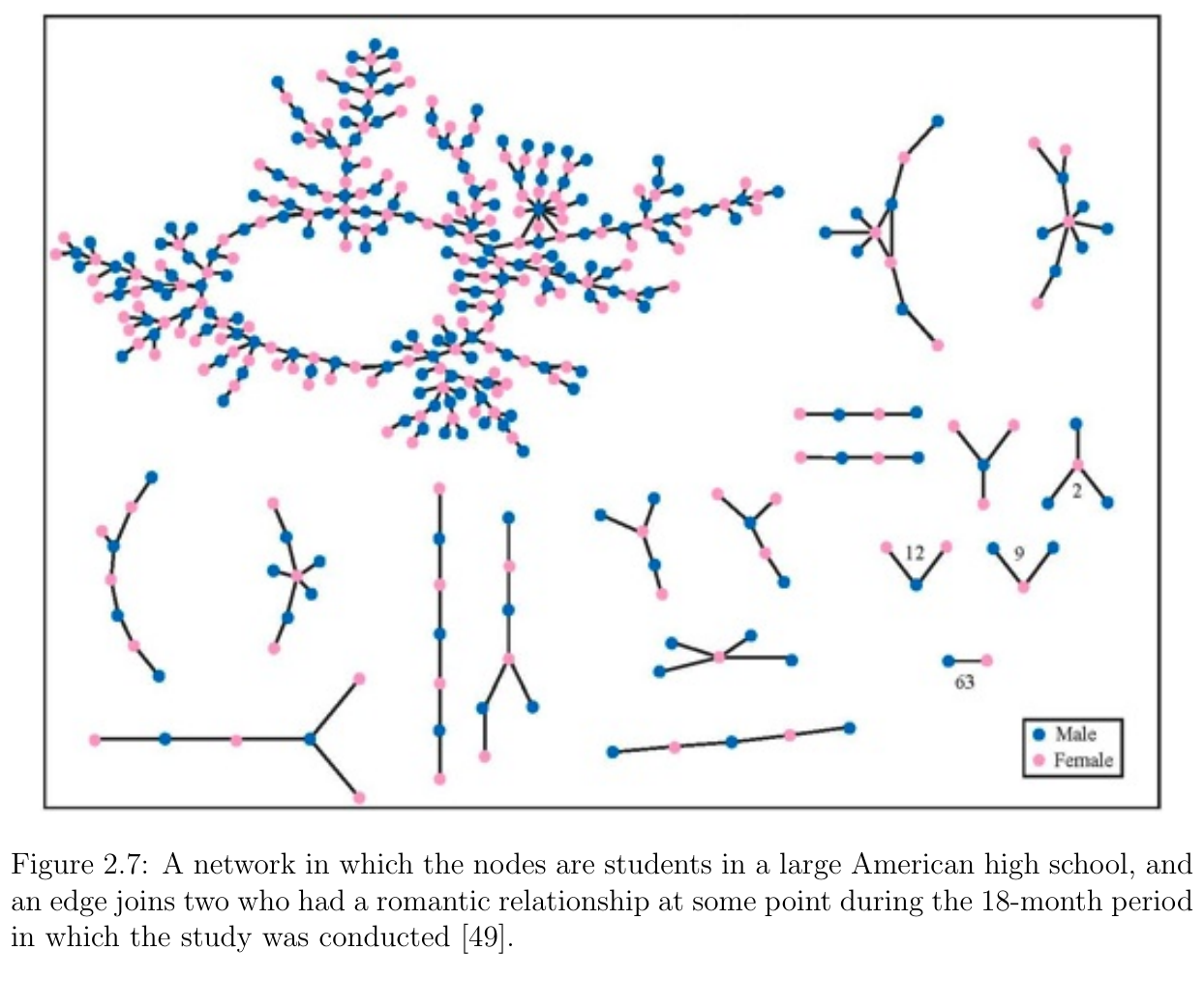
A component of a graph is a self-contained subset of the nodes
More precisely, a set of nodes is a component if
1. Every node in the subset has a path to every other node in the subset
2. The subset is not part of a larger set with property (1)
Example:

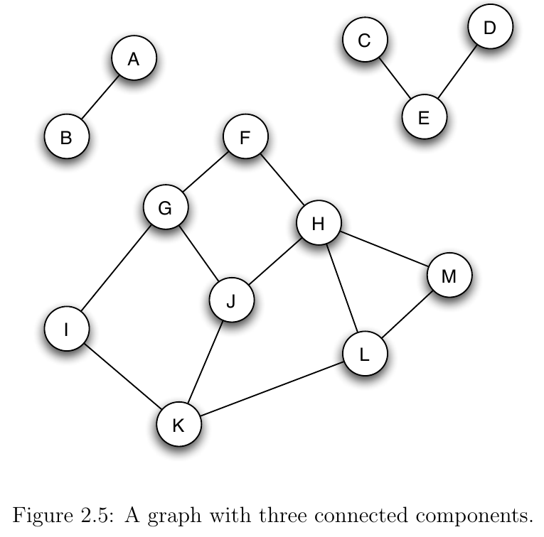
Finding Components¶

Graphs.jl provides functions to identify and work with components
connected_components(g) returns a vector of vectors, where each inner vector contains the nodes in one component
Let’s create a graph with multiple components and explore it

# Create a graph with three components
multi_component = SimpleGraph(10)
# Component 1: nodes 1, 2, 3
add_edge!(multi_component, 1, 2)
add_edge!(multi_component, 2, 3)
add_edge!(multi_component, 3, 1)
# Component 2: nodes 4, 5, 6, 7
add_edge!(multi_component, 4, 5)
add_edge!(multi_component, 5, 6)
add_edge!(multi_component, 6, 7)
add_edge!(multi_component, 7, 4)
# Component 3: nodes 8, 9
add_edge!(multi_component, 8, 9)
# Node 10 is isolated (its own component)

true

components = connected_components(multi_component)

4-element Vector{Vector{Int64}}:
 [1, 2, 3]
 [4, 5, 6, 7]
 [8, 9]
 [10]

println("Number of components: ", length(components))
for (i, comp) in enumerate(components)
    println("Component $i has $(length(comp)) nodes: $comp")
end

Number of components: 4
Component 1 has 3 nodes: [1, 2, 3]
Component 2 has 4 nodes: [4, 5, 6, 7]
Component 3 has 2 nodes: [8, 9]
Component 4 has 1 nodes: [10]

gplot(multi_component, nodelabel=1:10)

Why Components Matter¶

Components help us understand the structure of social networks
Each component represents a group that can communicate internally but not with other groups
In social network analysis, components reveal:
- Information silos: Ideas spread within components but not between them
- Echo chambers: Opinions reinforce within isolated groups
- Community detection: Natural groupings in social structures
- Influence boundaries: Limits of where influence can spread

Real-World Implications¶

Disease spread: Each component represents a boundary for transmission
- COVID-19 travel restrictions aimed to keep countries as separate components
- Contact tracing identifies components to contain outbreaks
Marketing: Products spread through word-of-mouth within components
- Need to seed each component separately for full market penetration
- Viral marketing campaigns can fail if they don’t bridge components
Political polarization: Separate components in social media
- Different groups may never see opposing viewpoints
- Bridging nodes between components become crucial for dialogue
Infrastructure resilience: Power grids, internet backbone
- Multiple components mean system fragmentation after failures
- Redundant connections prevent network from splitting into components

Giant Component¶

Many real-world networks have a giant component containing most nodes
Plus several small components or isolated nodes
Let’s check if ARPANET has this structure

arpa_components = connected_components(arpa)
println("ARPANET has $(length(arpa_components)) component(s)")
println("Component sizes: ", length.(arpa_components))

ARPANET has 1 component(s)
Component sizes: [13]

ARPANET is fully connected (one component) by design
This ensures any site can communicate with any other site
Network resilience was a key design goal for the early internet

Example¶

How many components are in this graph?

Real-World Network Examples¶

Let’s analyze some actual network datasets to see these concepts in practice
We’ll look at:
- Zachary’s Karate Club: A classic social network dataset
- Facebook ego networks: Social connections from real Facebook data
- Email networks: Communication patterns in organizations

Zachary’s Karate Club¶

Famous dataset from sociology (Zachary, 1977)
Documents friendships in a karate club that split into two factions
34 members (nodes), 78 friendships (edges)
Perfect for studying community structure and components

# Graphs.jl includes several famous networks as built-in datasets!
karate = smallgraph(:karate)

{34, 78} undirected simple Int64 graph

# Analyze the karate club network
using Statistics  # for `mean` function
println("Karate Club Network:")
println("  Nodes: ", nv(karate))
println("  Edges: ", ne(karate))
println("  Average degree: ", round(mean(degree(karate)), digits=2))
println("  Is connected: ", is_connected(karate))

Karate Club Network:
  Nodes: 34
  Edges: 78
  Average degree: 4.59
  Is connected: true

# Look at degree distribution
degrees = degree(karate)
println("\nDegree distribution:")
println("  Min degree: ", minimum(degrees))
println("  Max degree: ", maximum(degrees))
println("  Node with most connections: ", argmax(degrees))


Degree distribution:
  Min degree: 1
  Max degree: 17
  Node with most connections: 34

# Visualize the karate club network
gplot(karate, nodelabel=1:nv(karate), nodesize=0.1)

Exercise: Analyzing the Petersen Graph¶

The Petersen graph is a famous graph in graph theory
It appears in many theoretical results and counterexamples
Your task: analyze this network’s structure

# Load the Petersen graph
petersen = smallgraph(:petersen)

# TODO: Calculate the following properties
num_nodes = missing           # Total number of nodes
num_edges = missing           # Total number of edges
avg_degree = missing          # Average degree (should be the same for all nodes!)
is_it_connected = missing     # Is the graph connected?
is_it_tree = missing          # Is it a tree?
num_components = missing      # How many components?

# Print your results
println("Petersen Graph Analysis:")
println("  Number of nodes: ", num_nodes)
println("  Number of edges: ", num_edges)
println("  Average degree: ", avg_degree)
println("  Is connected: ", is_it_connected)
println("  Is it a tree: ", is_it_tree)
println("  Number of components: ", num_components)

Petersen Graph Analysis:
  Number of nodes: missing
  Number of edges: missing
  Average degree: missing
  Is connected: missing
  Is it a tree: missing
  Number of components: missing

Other Built-in Networks¶

Graphs.jl includes many classic networks for teaching and research
Some interesting examples you can explore:

# Examples of other built-in graphs
graphs_to_explore = [
    :house,        # The "house" graph (5 nodes)
    :bull,         # The bull graph
    :cubical,      # 3-dimensional cube
    :diamond,      # Diamond graph
    :dodecahedral, # Dodecahedron graph (20 nodes)
    :heawood,      # Heawood graph (14 nodes)
    :moebiuskantor,# Möbius-Kantor graph
    :octahedral,   # Octahedron graph
    :pappus,       # Pappus graph
    :tutte,        # Tutte graph (46 nodes)
]

# Try loading and analyzing one!
# Example: g = smallgraph(:house)

10-element Vector{Symbol}:
 :house
 :bull
 :cubical
 :diamond
 :dodecahedral
 :heawood
 :moebiuskantor
 :octahedral
 :pappus
 :tutte

Julia 2

Julia Package Development

Graph Theory 1

Strong and Weak Ties