Schelling Model with Agents.jl

Computational Analysis of Social Complexity

Prerequisites

Julia Basics (from week 2)
Julia Types (from week 2)
ABM intro

Outcomes

Learn to use the Julia REPL for running interactive ABM visualizations
Implement the Schelling segregation model using Agents.jl

References

Review Schelling Model¶

Recall the components of the Schelling segregation model
Environment: 25x25 grid of single family dwellings
Agents with properties:
- location (x,y) coordinate for current home
- type: orange or blue. Fixed over time. 250 of each
- happiness: 0 if less than $N$ of neighbors are of same type, 1 otherwise
Rules:
- Agents choose to move to unoccupied grid point if unhappy

Note neighbors for a particular cell are the the 8 other cells surrounding the cell of interest. Corner or edge cells have less than 8 neighbors

Agents.jl¶

We are now ready to get started implementing the Schelling segregation model in Julia
We’ll use the Agents.jl library, which is a very powerful ABM toolkit
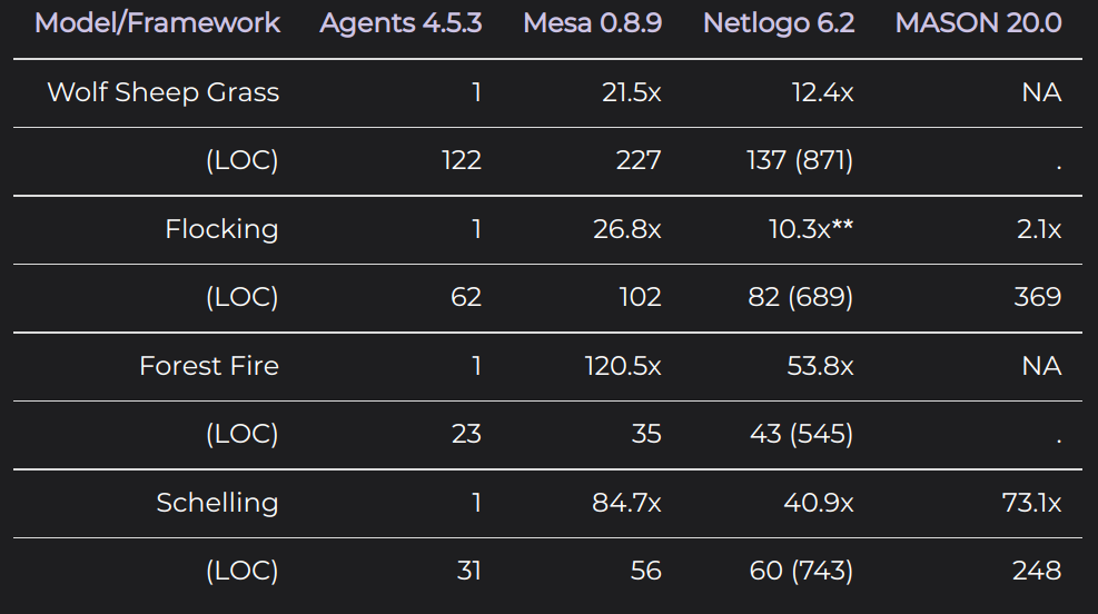
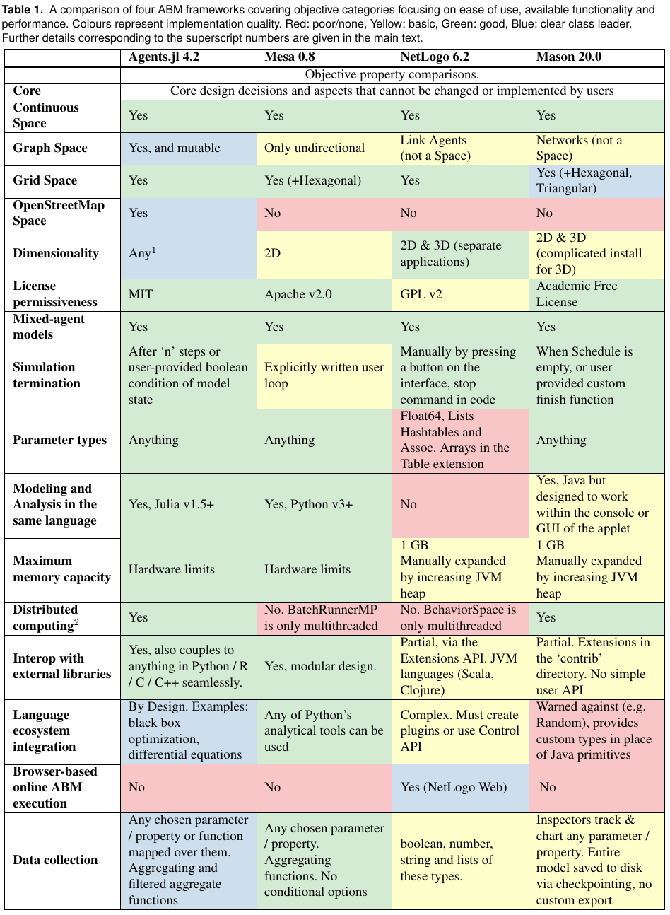
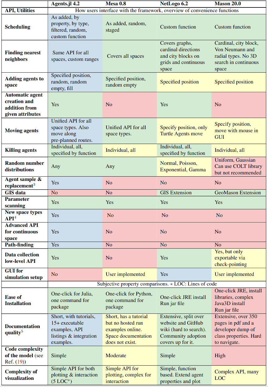
Here are some points of comparison between Agents.jl and other ABM software (from the Agents.jl website):

Schelling in Agents.jl¶

Let’s now implement the Schelling Segregation model in Agents.jl
The first thing we’ll need to do is define our Agent
The recommended way to do this is to create a new Julia struct using the @agent macro provided by Agents.jl
The macro will ensure a few things:
- The struct contains id and pos fields to keep track of the agent and its position
- The struct is mutable so the position can be updated
- The struct is a subtype of AbstractAgent so it can be used by other functions in Agents.jl

# load up packages we need for this example... might take a few minutes
# import Pkg
# Pkg.activate(".")
# Pkg.instantiate()

using Agents

@agent struct SchellingAgent(GridAgent{2})
    is_happy::Bool      # whether the agent is happy in its position. (true = happy)
    group::Int          # The group of the agent, determines mood as it interacts with neighbors 0: blue, 1: orange
end

We can see the complete structure of the ShellingAgent type using the dump function

dump(SchellingAgent)

SchellingAgent <: AbstractAgent
  id::Int64
  pos::Tuple{Int64, Int64}
  is_happy::Bool
  group::Int64

Schelling Environment¶

Our Schelling environment will be one the built-in Agents.jl spaces
We’ll use GridSpace

environment = GridSpaceSingle((25, 25); periodic = false)

GridSpaceSingle with size (25, 25), metric=chebyshev, periodic=false

Rules¶

The last part of our ABM that we need to specify is the rules for how agents respond to the environment and state
- Our rule is that agents will choose to move to an empty grid space if they have less than wanted_neighbors neighbors of the same group
Agents.jl requires us to implement these rules in a method agent_step!(agent::SchellingAgent, model)
We’ll make use of a couple helper functions provided by Agents.jl:
- move_agent_single!: move a single agent to an empty place in the environment. This modifies the pos field of the agent
- nearby_agents: return an array of all neighbors of a particular agent. This queries the pos field of all agents

function agent_step!(agent::SchellingAgent, model)
	want = model.wanted_neighbors
	have = 0
	for n in nearby_agents(agent, model)
		if n.group == agent.group
			have += 1
		end
	end
	agent.is_happy = have >= want
	if !agent.is_happy
		move_agent_single!(agent, model)
	end
	return
end

agent_step! (generic function with 1 method)

Combining Agents, Environment, and Rules¶

We now need to create an instance of the AgentBasedModel (or ABM for short) type
To construct our instance we need to specify our agent type, our environment, our rules (via agent_step! function), and any additional properties
These additional properties belong to the model, and can be thought of as parameters that should be calibrated
In our previous exposition we would have attached these to the environment

properties = Dict(:wanted_neighbors => 4)
schelling = AgentBasedModel(SchellingAgent, environment; properties=properties, agent_step! = agent_step!)

StandardABM with 0 agents of type SchellingAgent
 agents container: Dict
 space: GridSpaceSingle with size (25, 25), metric=chebyshev, periodic=false
 scheduler: fastest
 properties: wanted_neighbors

Add Agents¶

Now we have fully specified the behavior of our ABM, but we have a problem...
We don’t have any agents!!
To add agents, we’ll use the add_agent_single!(::SchellingAgent, model) function, which is provided by Agents.jl and knows how to place non-overlapping agents in our environment
- This will set the pos field for our agents
So that we can run many experiments, we’ll actually create a helper function that will create a new model from scratch and add agents to it

function init_schelling(;num_agents_per_group=250)
	environment = GridSpaceSingle((25, 25), periodic=false)
	properties = Dict(:wanted_neighbors => 4)
	model = ABM(SchellingAgent, environment; properties=properties, agent_step! = agent_step!)
	
	id = 0
	for group in 1:2, i in 1:num_agents_per_group
		agent = SchellingAgent(id+=1, (1, 1), false, group)
		add_agent_single!(agent, model)
	end
	model
end

model = init_schelling()

StandardABM with 500 agents of type SchellingAgent
 agents container: Dict
 space: GridSpaceSingle with size (25, 25), metric=chebyshev, periodic=false
 scheduler: fastest
 properties: wanted_neighbors

Running the Model¶

To run our model, we need to step forward in time
We do this using the step! function provided by Agents.jl
This function will iterate over all the agents in the model and call agent_step! for each of them

# advance one step
step!(model)

StandardABM with 500 agents of type SchellingAgent
 agents container: Dict
 space: GridSpaceSingle with size (25, 25), metric=chebyshev, periodic=false
 scheduler: fastest
 properties: wanted_neighbors

# advance three steps
step!(model, 3)

StandardABM with 500 agents of type SchellingAgent
 agents container: Dict
 space: GridSpaceSingle with size (25, 25), metric=chebyshev, periodic=false
 scheduler: fastest
 properties: wanted_neighbors

We can also use the run function
This function requires a model, agent_step! function, number of steps and array of agent property names to record
The output is a DataFrame with all the data

model = init_schelling()
adata = [:pos, :is_happy, :group]  # short for agent data
data, _ = run!(model, 10; adata)
data

Visualizing the Agents¶

One of the more instructive (and fun!) parts of agent based modeling is visualizing the data
To do this visualization we will use the abmplot function

using CairoMakie

agent_color(a) = a.group == 1 ? :blue : :orange
agent_marker(a) = a.group == 1 ? :circle : :rect
figure, _ = abmplot(model; agent_color, agent_marker, agent_size = 10)
figure # returning the figure displays it

Animating the Agents¶

We can also create a video that animates our agents moving throughout the system
We do this using the abmvideo function as follows

model = init_schelling();
abmvideo(
    "schelling.mp4", model;
    agent_color, agent_marker, agent_size = 10,
    framerate = 4, frames = 20,
    title = "Schelling's segregation model"
)

Interactive Application¶

Agents.jl also makes it very easy to create an interactive application for our model!
We can do this using the abmexploration function
This expects a single positional argument:
- model
We also have some keyword arguments
- params: Dict mapping model parameters to range of values to test
- agent_color, agent_marker, agent_size: control marker color color, symbol, and size as before
- adata: Array of (agent_property, summary_func) tuples that specify which data to plot in separate charts
- alabels: What label to put on the plots for adata

model = init_schelling()
adata = [(:is_happy, sum)]
alabels = ["n_happy"]
parameter_range = Dict(:wanted_neighbors => 0:8)
figure, abmobs = abmexploration(
    model;
    adata, alabels,
    agent_color, agent_marker, agent_size = 10,
    params=parameter_range,
)
figure

Running Julia Code in the REPL¶

In order to use the interactive app we need to run the code from the Julia REPL (not inside VS Code or Jupyter)
The REPL (Read-Eval-Print-Loop) is the default way to run Julia interactively
Let’s learn about the REPL before we run our interactive visualization

The Julia REPL¶

The REPL is typically started either by typing julia in a terminal or by clicking on the Julia icon in your Applications list
Once started, you will see a prompt julia> where you can enter Julia code
If you enter code and press Enter, the REPL will evaluate the code and print the result

REPL Modes¶

The REPL has several modes you can switch between:
1. Default mode julia>: Run Julia code and see output (default)
2. Shell mode shell>: Interact with underlying shell/terminal (activate with ;)
3. Help mode help?>: Get help on Julia functions (activate with ?)
4. Package mode pkg>: Manage Julia packages (activate with ])
To return to default mode from any other mode, press backspace at an empty prompt
Examples of what each mode prompt looks like:
- Default: julia>
- Shell: shell>
- Help: help?>
- Package: (@v1.9) pkg>

Running our Interactive Schelling Model¶

Now let’s run our interactive model from the REPL:
1. Open a terminal and type julia to start the REPL
2. Navigate to this notebook’s directory if needed (using ; for shell mode)
3. Copy and run the code from the cells above to set up the model
4. Run the interactive visualization code
5. You’ll be able to adjust parameters with sliders and see the model update in real-time!

Real-World Implications¶

Schelling’s model was groundbreaking for urban planning and social policy
Key insight: segregation doesn’t require intense prejudice - even mild preferences for similar neighbors create strong patterns
Applications beyond racial segregation:
- Income clustering in neighborhoods
- Social media echo chambers and political polarization
- Clustering in high school cafeterias
- Academic discipline segregation in universities
Model limitations: Reality includes housing costs, school quality, employment access, historical policies
Policy implication: Simply reducing prejudice may not eliminate segregation - structural interventions may be needed

Exercises¶

Exercise 1: Parameter Sensitivity Analysis¶

Using the interactive app or by modifying the code, explore how different wanted_neighbors values affect segregation:

Run the model with wanted_neighbors = 1 (agents want just 1 similar neighbor)
- Observe the final pattern. Is there segregation?
Run with wanted_neighbors = 3 (moderate preference)
- How does the pattern differ? How many steps to stability?
Run with wanted_neighbors = 6 (strong preference)
- What happens? Do all agents become happy?
Document your findings:
- At what threshold does segregation become noticeable?
- What happens when the threshold is too high?
- How does empty space (less than 500 agents total) affect the patterns?

Exercise 2: Model Extensions¶

Modify the Schelling model to explore these variations:

Three groups instead of two:
- Add a third group (e.g., green agents)
- What patterns emerge with three groups?
- Hint: Modify the init_schelling function to have for group in 1:3
Asymmetric populations:
- Try 400 agents of group 1 and 100 agents of group 2
- Does the minority group cluster more tightly?
- What happens to the majority group’s distribution?
Different happiness thresholds per group:
- Modify so group 1 wants 3 similar neighbors, group 2 wants 5
- Which group ends up more segregated?
- What does this suggest about tolerance and outcomes?
Distance-based happiness (Advanced):
- Instead of just counting similar neighbors, weight them by distance
- Immediate neighbors count as 1.0, diagonal neighbors as 0.7
- How does this change the segregation patterns?

Choose at least one modification to implement and document your observations.

ABM 1

Agent Based Models

ABM 2

Agent Based Models Review/Practice