Prerequisites
Introduction to Graphs
Weighted Graphs
Outcomes
Recall the key concepts of spectral theory from Linear Algebra
Desribe the key proprties of the Leintief family of production models
Explain the difference between “in”-based centrality and “out”-based centrality
Analyze the impact of sector specific shocks on other sectors of the US economy
References
QuantEcon Networks chapters 1-2 (especially section 1.2)
Linear Algebra
Linear algebra is the backbone of modern computational algorithms
Graphics
Statistics
Data analysis
Optimization
Machine Learning
Workhorse for accelerated computing
GPUs work on matrices to efficiently parallellize common computations
Specialty hardware like the TPU (tensor processing unit) take this even further
Building Blocks
Vectors: arrays of numbers representing points in multi-dimensional space
Matrices
Rectangular arrays that transform vectors
Also used to represent certain datasets/relationships: e.g. adjacency matrix in Graph Theory
Tensors: higher dimensional collections of numbers that allow high-dimensional
Vectors are 1d tensors, matrices 2d tensors, etc.
Implemented in numpy as
np.arrayand Julia as the build in array
Some Key Theories
Linear systems of equations
Inner product spaces (length, distance, and angles)
Eigenvalues and eigen vectors (spectral theory)
Spectral Theory
Let’s dig into eigenvalues and eigenvectors
Let
A scalar is an eigenvalue of if there exists a nonzero vector such that
A vector satisfying this equality is called an eigenvector corresponding to the eigenvalue
A vector sastifying is a left-eigenvector of
using LinearAlgebraA = [
0 -1
1 0
]
eigvals(A)2-element Vector{ComplexF64}:
0.0 - 1.0im
0.0 + 1.0imDefinitions
The set of all eigenvalues of is called the spectrum of and is written
The spectral radius of is written
The spectral radius important when considering the convergence of a dynamic system driven by
If and then the sequence is finite and will converge
Some facts (not proven here)
will have at most distinct eigenvalues
Eigenvectors are only unique to a scalar multiple: if is an eigenpair, then so is for any
Sometimes a matrix will have a repeated eigenvalue (the same value works with multiple distinct eigenvectors)
The algebraic multiplicity of an eigenvalue is the number of times it is repeated with distinct eigenvectors
An eigenvalue with an algebraic multiplicity of one is called simple
Diagonalization
A matrix is diagonalizable if
, is some invertible matrix
The decomposition is called the eigen decomposition or spectral decomposition of
The asymptotic properties of are determined by
Can be seen when is diagonalizable
If
Example: Worker Dynamics
Consider a continuum of workers (large number, not counted discretely)
Workers can be in one of two states: (1) employed and (2) unemployed
Each month employed workers become unemployed at rate , while unemployed workers are hired at rate
We express these dynamics as a weighted directed graph with adjacency matrix:
Row 1 gives the probabilities of employment and unemployement for an employed worker
Row 2 gives the probabilities of employment and unemployement for an unemployed worker
Transitions
Suppose we have a vector (2 element simplex) representing current fraction of workers that are employed and unemployed
Question... What matrix operation between and will give the fraction of workers that start next month as employed and unemployed?
alpha = 0.3
beta = 0.1

P = [1-alpha alpha; beta 1-beta]
2×2 Matrix{Float64}:
0.7 0.3
0.1 0.9x = [0.9, 0.1]2-element Vector{Float64}:
0.9
0.1# TODO: simulate for many periods# TODO: compare to largest left eigenvectorThe simulation should reveal the pattern summarized in Figure 1: repeated transitions move the population toward a steady state.
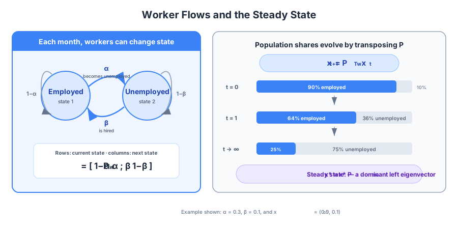
Figure 1:Worker transitions, the population update, and convergence to the dominant left eigenvector.
Neumann Series Lemma
We need one more linear alegbra result...
If and , then is non-singular and
This is known as the Neumann series lemma
Production Networks
We will now study a family of economic models that allow us to analyze the economy as a collection of sectors
These models were proposed by nobel prize winner Wassily Leontief in 1941 and are still commonly used today
The key idea behind a Leontief model is the input-output table
Input-output tables
Firms (companies) are categorized into distinct sectors
Firms use materials produced by other sectors as part of their production process
The relationship of flows of value are organized into an input/output table
| sector 1 | sector 2 | sector 3 | |
|---|---|---|---|
| sector 1 | |||
| sector 2 | |||
| sector 3 |
is called an input-output coefficient and is equal to:
Figure 2 connects this coefficient to both the production network and its matrix representation.
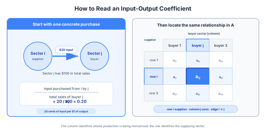
Figure 2:A coefficient records inputs flowing from supplier to buyer , normalized by buyer ’s total sales.
If is large, sector is an important supplier of intermediate goods to sector
The sum of column is the value of all inputs to sector
Row shows how intensively each sector uses good as an intermediate good
The input output table can be directly used as the adjacency matrix for a weighted directed graph
Input-output data
In the United States, the Bureau of Economic Analysis is responsible for compiling input-output tables for sectors
We’ll be studying the Input-Output Accounts Data
The main set of tables we’ll be using are called the
Make-UsetablesThe
Maketable shows the value of final goods produced by each sectorNote this is predominately a diagonal matrix as each sector primarily produces and sells final goods within their sector
Sometimes a firm will have secondary outputs as part of their production process
“Which industries produce which commodities?”
The
Usetables show the intermediate and final use of commodities across sectors“Who uses or consumes the commodities produced?”
using CSV, DataFrames, Graphs, SimpleWeightedGraphs, GraphPlot, ColorSchemes, Colors, Downloads, PlotlyBaseusing Downloads
function read_remote_csv(url)
bn = basename(url)
if !isfile(bn)
Downloads.download(url, bn)
end
CSV.read(bn, DataFrame)
end
make_15 = read_remote_csv("https://compsosci-resources.s3.amazonaws.com/graph-theory-lectures/data/QE-networks/make_15.csv");
use_15 = read_remote_csv("https://compsosci-resources.s3.amazonaws.com/graph-theory-lectures/data/QE-networks/use_15.csv");
codes = read_remote_csv("https://compsosci-resources.s3.amazonaws.com/graph-theory-lectures/data/QE-networks/codes.csv");Example: US 15 sector data
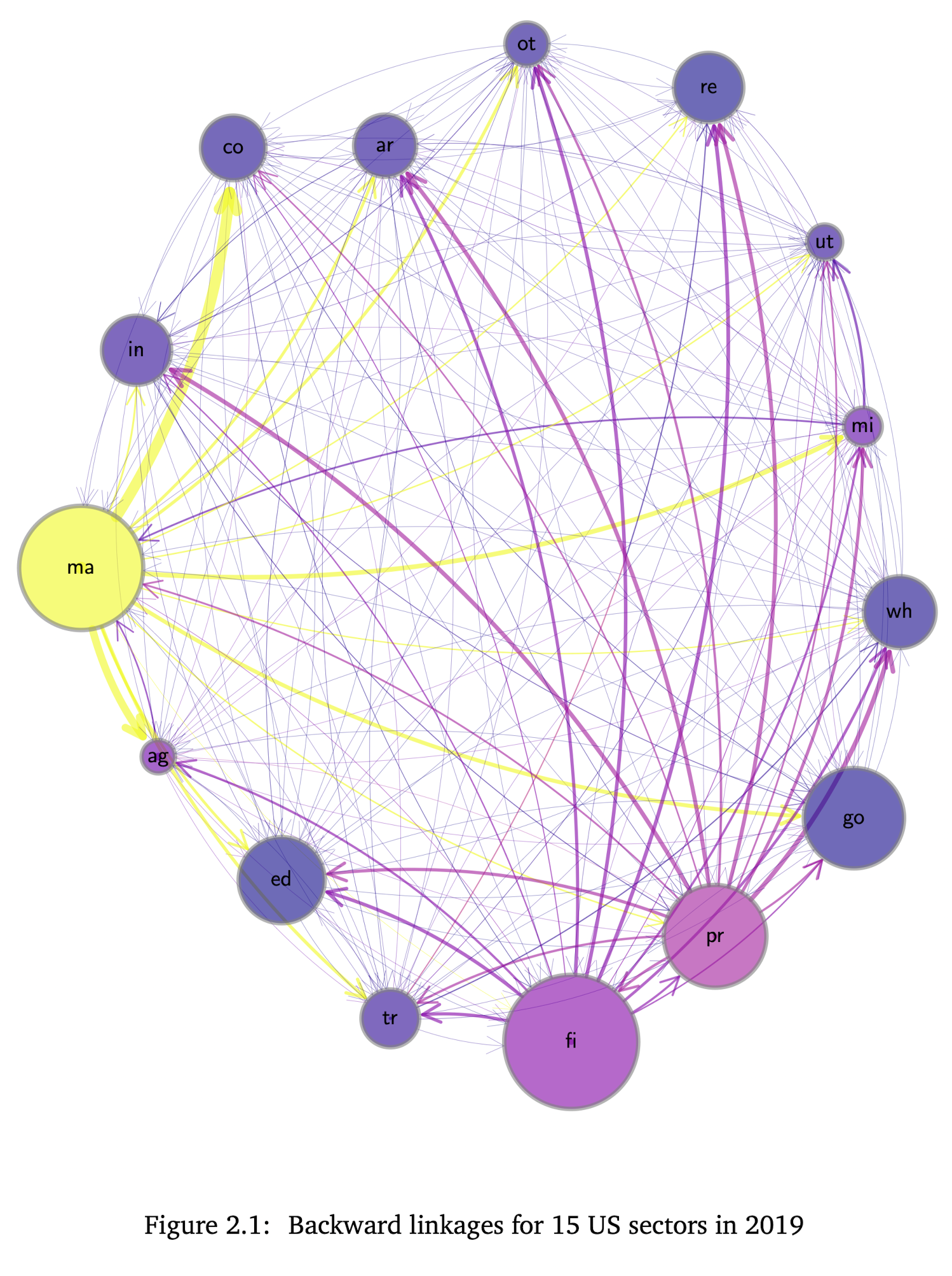
Color of nodes is according to their hub-based eigenvector centrality (see below)
Size of nodes is according to their total outputs (make table)
Thickness of edges is according to amount of goods
Represent and point from sector creating the intermediate good (sector ) to sector using intermediate good (sector )
Eigenvector Centrality
The node size above shows the hub-based eigenvector centrality
This is equal to the dominant eigenvector of the adjacency matrix (eigenvector associated with largest eigenvalue)
This measure of centrality measures the influence of a node in a network
When computing this statistic for a node
N, the value will be higher if it is connected to other “influential” nodes
Example
Let’s compute the eigenvector centrality for the data in the image above
I have some code to import the make/use files into a helpful struct
We’ll see what all the fields are as we progress through the lecture
to_int(x) = parse(Int, x)
to_int(x::Integer) = Int(x)

struct SectorData
    Z::Matrix{Int}
    X::Vector{Int}
    A::Matrix{Float64}
    F::Matrix{Float64}
    Z_df::DataFrame
    names::Vector{String}
    codes::Vector{String}
    N::Int
    G::SimpleWeightedDiGraph{Int64, Float64}
end

const CODES = let
    df = read_remote_csv("codes.csv")
    Dict(zip(df.name, df.code))
end

function load_sector(N)
    # read csv
    df = CSV.read("use_$(N).csv", DataFrame)

    # replace `---` with `0`
    df .= ifelse.(df .== "---", "0", df)

    # conver to int
    df[!, 2:end] .= to_int.(df[!, 2:end])

    # first column is industry name, next columns are sector values
    # first N rows are values
    Z = Array(df[1:N, 2:(N+1)])
    names = df[1:N, 1]
    codes = [CODES[n] for n in names]

    # total industry outputs come from teh `make_N.csv` file
    X = CSV.read("make_$(N).csv", DataFrame)[1:N, "Total Industry Output"]

    # value of sector j's inputs purchased from i / sales of `j`
    # or ...
    A = Z ./ X'

    F = Z ./ X

    # make copy of A where small values are set to zero to make plotting clearer
    A_copy = copy(A)
    A_copy[A .<= 0.01] .= 0;
    G = SimpleWeightedDiGraph(A_copy)

    SectorData(Z, X, A, F, df, names, codes, N, G)
end
load_sector (generic function with 1 method)data15 = load_sector(15);lambda15 = eigenvector_centrality(data15.G)15-element Vector{Float64}:
0.20015876206170186
0.15938537489092003
0.024488792126254755
0.01655605810501688
0.863307958233566
4.7179251777605e-17
9.919510282578063e-17
0.0160904862243379
0.03706307448992309
0.2744196179986345
0.33276423164786867
1.5167914026463714e-5
0.026176029930141512
0.0014956985704648131
0.00042398130095220904Plot(bar(x=data15.codes, y=lambda15))Accounting
Let...
be the final consumer demand for good
be total sales of sector
be inter-industry sales from sector to sector
Figure 3 shows how these quantities fit together before we write the accounting identity in matrix form.
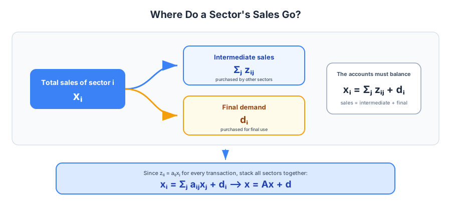
Figure 3:A sector’s sales split between intermediate sales and final demand; stacking the identities across sectors gives .
For accounts to add up we must have
Notice that
This means
Which can be written
Equilibrium
An equilibrium in a Leonteif model with input-output coefficient matrix and a vector of final consumer demands for each sector is a vector for sector-specific output such that is satisfied
Note that and are treated as given
To find this vector requires that we trace the impact of final demand on the intermediate linkages through
Example:

Example
Suppose
Will cause 3 to consume more from its suppliers (2 and 4)
Which will cause 2 to demand more from 1
Which will cause 1 to demand more from 2 and 4
... and so on
Computing an equilibrium is not entirely straight forward...
Computing an Equilibrium
Define as the value added by sector
Assumption: The input-output adjacency matrix satisfies
This holds whenever
When this assumption holds, for each there is a unique, nonnegative output solution given by
The matrix is called the Leontief inverse associated with the coefficient matrix
L15 = inv(I - data15.A)

# propose a demand vector where each element is between [100, 600]
d = rand(15).* 500 .+ 100

L15 * d
15-element Vector{Float64}:
529.5876385695651
539.6471159147281
504.4562459246958
213.10961424757355
1684.102232985288
490.039956568086
363.5297064550896
418.5497166984117
443.79727522648716
750.0649628686189
1149.3512051482644
303.1862869553239
192.75063112958023
476.7757695206679
337.41500397173866Question
We don’t have a field for d in our SectorData struct.
How could we compute/derive d given the fields we do have?
fieldnames(SectorData)(:Z, :X, :A, :F, :Z_df, :names, :codes, :N, :G)Demand Shocks
A common form of economic analysis is to consider the impact of external “shocks”
Often, these are modeled as a one time change in the value of a variable
Let’s consider a demand shock of size such that demand moves from to
The equilibrium vector shifts from to
Define
What happens between the initial change in demand and the final change in output? Figure 4 traces the response one round at a time.
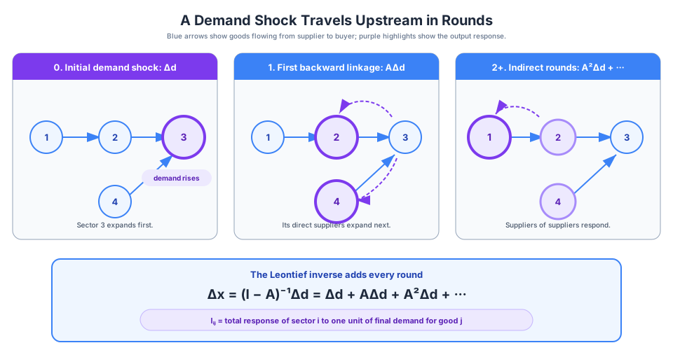
Figure 4:A demand shock propagates upstream through direct and indirect suppliers; the Leontief inverse accumulates every round of the response.
NSL
We will further assume that so that we can write the expression for as an infinite sum using the Neumann Series Lemma:
is the initial response in each sector,
is the response generated by the first round of backward linkages,
is the response generated by the second round, and so on.
The total response is the sum of the responses at each round
The typical element of shows total impact on sector i of a unit change in the demand for good
L1515×15 Matrix{Float64}:
1.29184 0.013976 … 0.021353 0.0081746 0.0192996
0.0298015 1.14899 0.0146944 0.00990947 0.0300173
0.0172818 0.0233041 0.0316325 0.00965223 0.0183746
0.0070151 0.00826026 0.00638848 0.00764268 0.0342044
0.406849 0.24425 0.190964 0.136599 0.286737
0.0044889 0.0013509 … 0.00111709 0.000775398 0.00129499
7.51567e-8 7.41503e-8 3.39839e-7 2.05879e-5 3.82796e-7
0.00610972 0.00983046 0.0116882 0.00995762 0.0189601
0.00518775 0.00943438 0.0271543 0.0277547 0.0459451
0.107845 0.0933879 0.147118 0.131159 0.120384
0.0462756 0.134203 … 0.201764 0.114416 0.159921
0.000123414 0.000127331 0.00356867 0.00797317 0.0142819
0.00422839 0.00511009 1.03468 0.0154229 0.0140417
0.00369676 0.00364725 0.0167158 1.01266 0.0188287
0.000730455 0.000825878 0.00497073 0.00307743 1.00398Plot(heatmap(z=L15))