Game Theory 1

Computational Analysis of Social Complexity
Fall 2025, Spencer Lyon

Prerequisites

Julia basics

Outcomes

Understand the basic structure of a Game
Be able to identify any Nash Equilibria in pure strategies for a normal form game
Understand how normal form and extensive form games are related

References

Easley and Kleinberg chapter 6

Introduction¶

Computational social science analyzes the connectedness of natural, social, and technological systems
Graph theory (networks) has helped us understand how the structure of relationships influence outcomes
We now turn to how behaviors, incentives, and strategies influence choices (and thus outcomes)
The study of how entities make strategic choices in settings where outcomes depend on individual choices and the choices of others is called game theory
Game theory is a very rich topic at the intersection of mathematics and economics
We will study key concepts, but will not cover them in detail or exhaustively

What is a Game?¶

A game is a description of a strategic environment composed of three elements:
1. A finite set of $N$ players
2. For each player $i$ , a set of feasible actions $S_i$
  - Define $\Sigma = \times_i S_i$ as action space and $\sigma$ as typical element
3. For each player $i$ , a payoff function $p_i:\Sigma \rightarrow \mathbb{R}$
To help with notation we’ll focus on two player games (N=2)
We’ll also start by considering that each player has a discrete set of actions (WLOG call them $1 \dots M_i$ for player $i$ )
Basic concepts and definitions can be naturally extended to cases where $N>2$

Example: Prisoner’s Dilemma¶

A very famous example of a game is called the prisoner’s dilemma
Story: two robbery suspects brought in for questioning
Investigator immediately separates them and gives both the same deal

If you confess and your partner doesn’t, you go free and he gets 10 years. If you both confess you each get 4 years, and if neither confesses you each get 1 year.

The payoffs for this game can be summarized as follows:

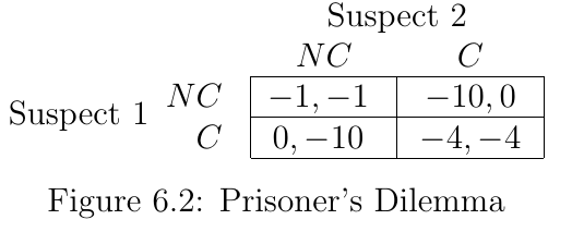
Each table entry has two items
In terms of our definition of a game we have...
- N = 2 players
- Strategys: $S_i = \{\text{not confess}, \text{ confess} \}$ for both players
- Payoffs $p_i$ as specified in the table

Payoffs as matrices¶

A common representation of payoffs for a single player is a matrix called the payoff matrix $P_i \in \mathbb{R}^{M_1 \times M_2}$
The row i, column j element gives the payoff when player i chooses the $i$ th action in $S_1$ and player j chooses the $j$ th action in $S_2$
For the Prisoner’s Dilemma game above, we have

pd_p1 = [-1 -10; 0 -4]
pd_p2 = [-1 0 ;-10 -4]

2×2 Matrix{Int64}:
  -1   0
 -10  -4

Best Responses¶

What would happen in the Prisoner’s dilemma game?
You may think that these partners in crime would like to stick together and get a total of 1 year each by not confessing
However, that doesn’t happen
The investigator knows game theory and rigged the game against them...

What should Suspect 1 Do?¶

Let’s consider suspect 1

pd_p1

2×2 Matrix{Int64}:
 -1  -10
  0   -4

Suppose suspect 1 believes suspect 2 will not confess
- Suspect 1 now faces the first column of pd_p1 and sees he’s better of confessing and getting 0 years instead of -1
What if suspect 1 believes suspect 2 will confess?
- 1 now faces second column and prefers -4 to a -10, so he still chooses to confess
In either case, suspect 1’s best response is to confess
Because confess is always a best response, we call it a dominating strategy (in this strictly dominating because it is always strictly better than not confess)

How about Suspect 2?¶

If we look closely at suspect 2’s payoffs we see his game is symmetric to suspect 1’s:

pd_p2

2×2 Matrix{Int64}:
  -1   0
 -10  -4

No matter what suspect 1 chooses, suspect 2’s best response is to confess
The rational outcome is that both players confess and spend 4 years together in prison

Nash Equilibrium¶

How did this happen? How is it a rational outcome i.e. an equilibrium?
A famous concept in game theory is called Nash equilibrium (after famous economist John Nash)
Definition: A strategy $\sigma$ is a Nash equilibrium if $\sigma_i$ is a best response to $\sigma_{-i}$ (everyone else’s actions)
Intuition: A strategy is an Nash equilibrium if after taking into account every one else’s strategies, each player does not want to change their own

Computing Nash Equilibria¶

There are various algorithms that we can use for computing Nash equilibria
Fow now we will utilize the implementation of these algorithms in the GameTheory.jl package
Let’s load it up and create a version of our prisoner’s dilemma game:

# import Pkg; Pkg.add("GameTheory")

using GameTheory

p1 = Player(pd_p1)

2×2 Player{2, Int64}:
 -1  -10
  0   -4

GameTheory.jl requires that payoff matrices are always specified from the perspective of the current player
This means that we need to “reorient” suspect 2’s payoffs such that his actions are noted on the rows
Becuase this is a symmetric game, suspect 2’s payoffs from suspect 2’s perspective looks exactly the same as suspect 1’s payoffs from suspect 1’s perspective
We can construct our NormalFormGame with two copies of the p1 player above

pd_g = NormalFormGame([p1, p1])

2×2 NormalFormGame{2, Int64}

We can now ask GameTheory.jl to compute the nash Equilibria for us
We’ll use the pure_nash function to do this (we’ll talk about what “pure” means soon)

pd_eq = pure_nash(pd_g)

1-element Vector{Tuple{Int64, Int64}}:
 (2, 2)

As we said before, the only equilibrium outcome to this game is that they both confess
We can see the payoffs each player gets in equilibrium by “indexing” into the game using the strategy array
The two expressions below are equivalent in this case

pd_g[pd_eq[1]...]

2-element Vector{Int64}:
 -4
 -4

# ↑ Equivalent to ↓
pd_g[2, 2]

2-element Vector{Int64}:
 -4
 -4

Non symmetric games¶

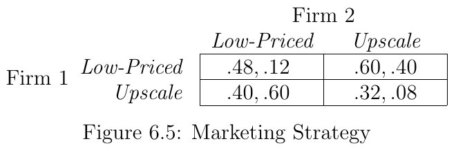
Not all games are symmetric like the prisoner’s dilemma
Consider the following game
- Two players (firms) and two strategies each (sell low price or upscale goods)
- 60% of total spending comes from people who prefer low prices
- Firm 1 more popular, so when they compete in same segment, firm 1 gets 80% of market
Below you find the payoff matrix in units of “% of total possible profit”

Strategies¶

Firm 1 has a dominant strategy: low-priced. They will always play this strategy
Firm 2 is less clear:
- If firm 1 were to choose the upscale market, they would be better off choosing low-priced
- however, when firm 1 chooses low-priced, firm 2 best response is upscale
How to find equilbirum?

Iterated Deletion of Dominated Strategies¶

An algorithm that can help find the solution to this game is called iterated deletion of dominated strategies
The algorithm proceeds as follows:
- Set iteration $n = 0$
- Let $S_i^n$ be set of remaining actions for player $i$ on iteration $n$ . Start $S_i^0 = S_i$
- On iteration $n$ , for each player $i$ remove from $S_i^n$ any strategies that are dominated by other strategies in $S_i^n$ (taking into account $S_{-i}^n$ ). Call surviving strategies $S_i^{n+1}$
- Repeat for all players $i$
- Repeat until one of two conditions is met:

Each player has only one remaining strategy: $|S_i^{n+1}| = 1 \forall i$ -- this is NE
One or more players has an empty strategy set

Application to Marketing Game¶

Applying this algorithm we start with $S_1^0 = \{1, 2\} \; S_2^0 = \{1, 2\}$
We see form firm 1 it is optimal to play strategy 1 for any choice of firm 2, which causes us to delete 2. Now we have $S_1^1 = \{1 \} \; S_2^1 = \{1, 2\}$
Now firm 2 takes into account that 1 will play 1 -- only best response is to play 2 and we get $S_1^2 = \{1 \} \; S_2^2 = \{2\}$
We are done!
The unique Nash Equilibrium is for firm 1 to take the low-price segment and firm 2 to take the upscale segment

Exercise¶

Construct the Marketing Game using GameTheory.jl
Verify that the only pure strategy nash equilibrium is [1, 2]
HINT: don’t forget to write player 2’s payoffs from player 2’s perspective!

p1_market = Player([0.0 0; 0 0])
p2_market = Player([0.0 0; 0 0])
g_market = NormalFormGame([p1_market, p2_market])

2×2 NormalFormGame{2, Float64}

Matching Pennies¶

Consider the payoff matrices for another famous game called Matching Pennies

pennies_p1 = [-1 1; 1 -1]
pennies_p2 = [1 -1; -1 1]

pennies_p1, pennies_p2

([-1 1; 1 -1], [1 -1; -1 1])

Question: how many players are there?
How many strategies does player 1 have? Player 2?

Pure Strategies¶

Choosing a strategy outright is called playing a pure strategy
Neither player will always choose H or T no matter what the other player does
We can say that there is no Nash Equilibrium in pure strategies
However, for all games we will consider (and most games in general) there is always a Nash equilibrium...

Mixed Strategies¶

Sometimes players will not be able to play pure strategies in eqiulibrium
In these cases they will need to randomize their behavior
A mixed strategy is a probability distribution over strategies
For example, in the matching pennies game, a mixed strategy is to play H with probabilty 0.5 and T with probability 0.5
It turns out that both players playing this mixed strategy is the unique Nash Equilibrium of the matching pennies game
Intuition: Why does 50-50 randomization work? In equilibrium, each player makes their opponent indifferent between their choices. If player 1 plays H or T with 50% probability each, then player 2’s expected payoff is the same whether they choose H or T (both give expected payoff of 0). This mutual indifference is what sustains the equilibrium - neither player has an incentive to deviate from their randomization.

Mixed Strategies with GameTheory.jl¶

GameTheory.jl can compute mixed strategy nash equilibria for us
To do that we’ll use the support_enumeration method (support enumeration is the name of an algorithm for computing all NE of a game, in pure or mixed strategies)

Bimatrix¶

Before we have GameTheory compute our mixed strategy NE, we’ll show one other way to create a NormalFormGame -- with a payoff bimatrix
For an $N$ player game with $N_i$ strategies for each player, a bimatrix is an $N_1 \times N_2 \times \cdots \times N_N \times N$ array of payoffs
For our game, we need a 2x2x2 array
- last 2 represents 2 players
- first two 2’s represent 2 actions per player

pennies_bimatrix = zeros(2, 2, 2)
pennies_bimatrix[1, 1, :] = [-1, 1]
pennies_bimatrix[1, 2, :]  = [1, -1]
pennies_bimatrix[2, 1, :] = [1, -1]
pennies_bimatrix[2, 2, :] = [-1, 1]
pennies_g = NormalFormGame(pennies_bimatrix)

2×2 NormalFormGame{2, Float64}

Notice how when using a bimatrix we can directly read the cells of the normal form game
- The (H,H) cell is in position [1,1] and has payoffs [-1, 1]
- The (T, H) cell is in position [2, 1] and has payoffs [1, -1]
- etc.
This can make it easier to specify payoffs because we don’t have to worry about “player N payoffs from player N’s perspective”

support_enumeration(pennies_g)

1-element Vector{Tuple{Vector{Float64}, Vector{Float64}}}:
 ([0.5, 0.5], [0.5, 0.5])

Exercise¶

Try support_enumeration with the other two games we’ve worked with
- What does it give you with the prisoner’s dilemma?
- What does it give you with the marketing game?

# TODO: your code AND explanation here

ABM 2

Academic Paper Virality: An Agent-Based Model

Game Theory 1

Network Traffic with Game Theory

Introduction¶

What is a Game?¶

Example: Prisoner’s Dilemma¶

Payoffs as matrices¶

Best Responses¶

What should Suspect 1 Do?¶

How about Suspect 2?¶

Nash Equilibrium¶

Computing Nash Equilibria¶

Non symmetric games¶

Strategies¶

Iterated Deletion of Dominated Strategies¶

Application to Marketing Game¶

Exercise¶

Matching Pennies¶

More Questions¶

Pure Strategies¶

Mixed Strategies¶

Mixed Strategies with GameTheory.jl¶

Bimatrix¶

Exercise¶