Network Traffic with Game Theory

Computational Analysis of Social Complexity
Fall 2025, Spencer Lyon

Prerequisites

Networks
Game Theory

Outcomes

Represent network traffic weighted DiGraph
Analyze equilibrium network outcomes using the concept of Nash Equilibirum
Understand Braes’ paradox
Learn about the concept of social welfare and a social planners

References

Easley and Kleinberg chapter 8

Congestion¶

We regularly use physical networks of all kinds
- Power grids
- The internet
- Streets
- Railroads
What happens when the networks get congested?
- Typically -- flow across the network slows down
Today we’ll study how game theoretic ideas are helpful when analyzing how a network with finite capacity or increasing costs

A Traffic Network¶

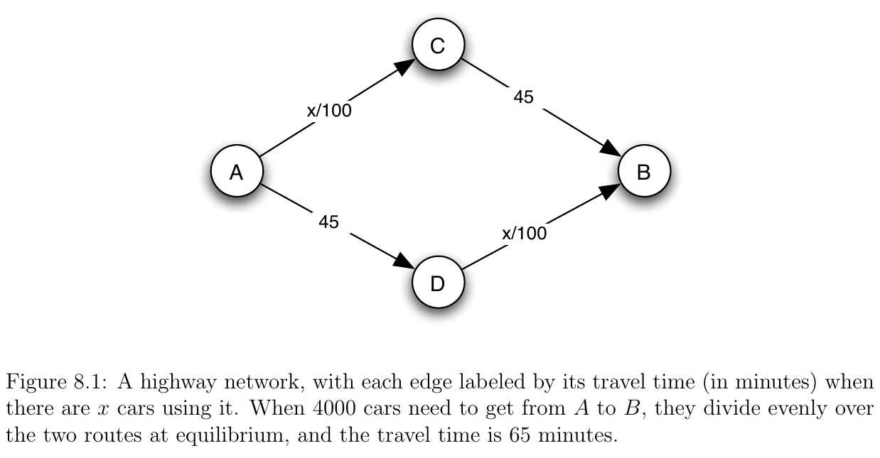
We’ll start by considering a traffic network
The figure caption has extra detail -- so be sure to read it!

We’ll write up some helper Julia functions that will let us create and visualize the traffic network for arbitrary values of x

using Graphs, SimpleWeightedGraphs, GraphPlot

function traffic_graph1(x)
    A = [
        0 0 x/100 45;
        0 0 0 0;
        0 45 0 0;
        0 x/100 0 0
        ]
    SimpleWeightedDiGraph(A)
end

traffic_graph1 (generic function with 1 method)

function plot_traffic_graph(g::SimpleWeightedDiGraph)
    locs_x = [1.0, 3, 2, 2]
    locs_y = [1.0, 1, 0, 2]
    labels = collect('A':'Z')[1:nv(g)]
    gplot(g, locs_x, locs_y, nodelabel=labels, edgelabel=weight.(edges(g)))
end

plot_traffic_graph (generic function with 1 method)

plot_traffic_graph(traffic_graph1(10))

Try changing the argument to traffic_graph1 to see how the network changes

The Game¶

Now suppose, as indicated in the figure caption, that we have 4,000 drivers that need to commute from A to B in the morning
If all take the upper route (A-C-B) we get a total time of 40 + 45 = 85 minutes
If all take the lower route (A-D-B) we get a total time of 40 + 45 = 85 minutes
If, however, they evenly divide we get a total time of 20 + 45 = 65 minutes

Equilibrium¶

Recall that for a set of strategies (here driving paths) to be a Nash Equilibrium, each player’s strategy must be a best response to the strategy of all other players
We’ll argue that the only NE of this commuting game is that 2,000 drivers take (A-C-B) and 2,000 take (A-D-B) and everyone takes 65 minutes to commute

Exercise¶

Show that this strategy (2,000 drivers take (A-C-B) and 2,000 take (A-D-B)) is indeed a Nash equilibrium
To do this recognize that the game is symmetric for all drivers
Then, argue that if 3,999 drivers are following that strategy, the best response for the last driver is also to follow the strategy

Numerical Verification¶

Let’s verify why the 50-50 split is indeed an equilibrium:

Current equilibrium: 2,000 drivers on each path, everyone takes 65 minutes

If you’re driver #2,001 considering which path to take:

If you join the upper path (A-C-B):
- Edge A-C now has 2,001 drivers: 2,001/100 = 20.01 minutes
- Edge C-B still takes 45 minutes
- Total time: 20.01 + 45 = 65.01 minutes
If you join the lower path (A-D-B):
- Edge A-D now has 2,001 drivers: 2,001/100 = 20.01 minutes
- Edge D-B still takes 45 minutes
- Total time: 20.01 + 45 = 65.01 minutes

Result: Both paths give the same travel time! No driver has an incentive to switch paths. This confirms our Nash equilibrium.

Your work HERE!

Discussion¶

Note a powerful outcome here -- without any coordination by a central authority, drivers will automatically balance perfectly in equilibrium
The only assumptions we made were:
1. Drivers want to minimize driving time
2. Drivers are allowed to respond to the decisions of others
The first assumption is very plausable -- nobody wants to sit in more traffic than necessary
The second highlights a key facet of our modern society...
- Information availability (here decisions of other drivers) can (and does!) lead to optimal outcomes without the need for further regulation or policing

function traffic_graph2(x) G = traffic_graph1(x) # Add an edge with minimal weight (1e-16 instead of 0) because # GraphPlot doesn’t display edges with weight 0 add_edge!(G, 3, 4, 1e-16) G end

function traffic_graph2(x)
    G = traffic_graph1(x)
    # need to add an edge with minimal weight so it shows up in plot
    add_edge!(G, 3, 4, 1e-16)
    G
end

traffic_graph2 (generic function with 1 method)

plot_traffic_graph(traffic_graph2(10))

Exercise¶

Is a 50/50 split of traffic still a Nash equilibrium in this case?
Why or why not?
Is all 4,000 drivers doing (A-C-D-B) a Nash equilibrium?
Why or why not?

Braess’ Paradox¶

In the previous exercise, we saw a rather startling result...
Doing a network “upgrade” -- adding a wormhole connecting C and D -- resulted in a worse equilibrium outcome for everyone!
The equilibrium driving time is now 80 minutes for all drivers instead of 65 minutes (which was the case before the wormhole)
This is known as Braess’ paradox

Real-World Examples¶

Braess’ paradox is not just theoretical - it has been observed in real traffic networks:

New York City (1990): When 42nd Street was closed for Earth Day, traffic flow actually improved rather than worsened. The city later made some closures permanent.
Stuttgart, Germany (1969): After investing in a new road to ease congestion, traffic conditions worsened. The road was eventually removed, restoring better traffic flow.
Seoul, South Korea (2003): The demolition of the Cheonggyecheon highway led to improved traffic conditions, contrary to predictions of chaos.

These cases demonstrate that sometimes removing network capacity can lead to better equilibrium outcomes - a counterintuitive result that game theory helps us understand!

Follow ups¶

Braess’ paradox was the starting point for a large body of research on using game theory to analyze network traffic
Some questions that have been asked are:
- How much larger can equilibrium travel time increase after a network upgrade?
- How can network upgrade be designed to be resilient to Braess’ paradox?

Many economic models are composed of individual actors who make autonomous decisions and have autonomous payoffs
We’ve been studying some of these settings using tools from game theory, focusing on the individual perspective
- Our notion of equilibrium is dependent on no individual wanting to change strategy in response to other strategies
Another form of analysis works at the macro level -- we analyze the total payoff for all agents (i.e. sum of payoffs)
We call this aggregate payoff social welfare

In an economic model, someone who seeks to maximize social welfare is called a social planner
A social planner is given the authority to make decisions for all agents
In our traffic model, a social planner would choose to ignore the wormhole and have 1/2 the drivers take A-C-B and the other half take A-D-B
- In this case everyone would be better off with a cost of 65 minutes instead of the equilibrium 80 minutes

Cost of Freedom¶

Question: in a generic traffic model, how much worse can the equilibrium outcome be than the social optimum?
In our example,
- Optimal social welfare is 4000 * 65 = 260,000 total minutes
- Equilibrium social welfare is 4000 * 80 = 320,000 total minutes
- A change of 60,000 total minutes
Price of Anarchy: This ratio of equilibrium cost to optimal cost is formally called the Price of Anarchy
- Price of Anarchy = Worst Nash Equilibrium Cost / Social Optimum Cost
- In our example: PoA = 320,000 / 260,000 = 1.23 (the equilibrium is 23% worse than optimal)
To answer this question for a general traffic model, we need to be able to compute the equilibrium for a generic traffic model
We may study this next week, or perhaps even on your homework 😉

Game Theory 1

Game Theory 2

More Game Theory

Network Traffic with Game Theory

Congestion¶

A Traffic Network¶

The Game¶

Equilibrium¶

Exercise¶

Numerical Verification¶

Discussion¶

Exercise¶

Braess’ Paradox¶

Real-World Examples¶

Follow ups¶

Social Welfare¶

The Social Planner¶

Cost of Freedom¶