Ignition: Chicken-and-Egg, Lock-In, and Tipping

Computational Analysis of Social Complexity
Fall 2026, Spencer Lyon

Prerequisites

Platforms and Matchmakers
Game theory (week 8)
ABM concepts (week 6)
Graphs (week 3)

Outcomes

Model the chicken-and-egg problem as a coordination game with multiple equilibria
Simulate increasing-returns adoption and explain lock-in and path dependence
Analyze threshold adoption on networks and identify tipping conditions
Evaluate when winner-take-all does and does not apply

References

Easley & Kleinberg, Chapter 19: Cascading Behavior in Networks (required)
Arthur (1989), Competing Technologies, Increasing Returns, and Lock-In by Historical Events
Matchmakers (Evans & Schmalensee, 2016), Chapter 5 (optional extra reading)

using GameTheory
using Graphs
using Plots
using Random
using Statistics

Two Platforms Walk into a Market¶

OpenTable launched in 1998 with a problem
- Diners would not visit a reservation platform with no restaurants
- Restaurants would not buy into a platform with no diners
Its response was intensely local
- Install reservation terminals in San Francisco restaurants
- Make the service free for diners
- Build enough density in one city, then repeat
OpenTable ignited

A Second Story¶

Windows Phone launched in 2010
Microsoft spent billions and reviewers praised much of the hardware
But users asked: where are the apps?
Developers asked: where are the users?
No apps $\rightarrow$ no users $\rightarrow$ no apps
By 2017, the platform was effectively dead

The Tension¶

Same chicken-and-egg problem
Opposite outcomes
Recall from Platforms and Matchmakers:
- Same-side network effects connect participants on one side
- Cross-side network effects connect activity across sides
What separates ignite from fizzle?
Today we study three answers: equilibrium selection, increasing returns, and network structure

Build 1: Chicken-and-Egg as a Game¶

Let the two players be Restaurants and Diners
Each chooses one action: Join or Stay out
Joining together creates value for both sides
Joining alone is costly
Staying out is safe, but produces no platform value
Before calculating anything: what outcomes seem self-reinforcing?

Payoffs¶

Rows are the Restaurant’s action: Join, then Stay out
Columns are the Diner’s action: Join, then Stay out
Each cell reports (Restaurant, Diner)

\begin{array}{c|cc} & \text{Diner: Join} & \text{Diner: Stay\ out} \\ \hline \text{Restaurant: Join} & (3,3) & (-2,0) \\ \text{Restaurant: Stay\ out} & (0,-2) & (0,0) \end{array}

(1)

The numbers are illustrative; their ordering carries the economics

restaurant_payoffs = [3 -2; 0 0]
diner_payoffs = [3 -2; 0 0]

restaurant = Player(restaurant_payoffs)
diner = Player(diner_payoffs)
platform_game = NormalFormGame([restaurant, diner])

2×2 NormalFormGame{2, Int64}:
 (3, 3)   (-2, 0)
 (0, -2)  (0, 0)

Recall from Week 8: Use Best Responses¶

If Diners join, the Restaurant’s best response is to join: $3 > 0$
If Diners stay out, the Restaurant’s best response is to stay out: $0 > -2$
The Diner faces the same logic
A Nash equilibrium is an action profile in which both actions are best responses
Question: can there be more than one?

coordination_equilibria = pure_nash(platform_game)

[(actions = eq, payoffs = platform_game[eq...]) for eq in coordination_equilibria]

2-element Vector{@NamedTuple{actions::Tuple{Int64, Int64}, payoffs::Vector{Int64}}}:
 (actions = (1, 1), payoffs = [3, 3])
 (actions = (2, 2), payoffs = [0, 0])

Reveal: The Bad Outcome Is Also an Equilibrium¶

(Join, Join) is a Nash equilibrium
(Stay out, Stay out) is also a Nash equilibrium
this figure marks both equilibria and the best-response arrows that sustain each one
At the bad equilibrium, neither side wants to join alone
The good equilibrium is Pareto-superior, but that does not make beliefs coordinate on it
A platform’s first job is therefore equilibrium selection
Critical mass is the participation level beyond which joining becomes self-sustaining

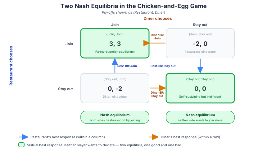
Bimatrix of the chicken-and-egg game with best-response arrows showing two Nash equilibria — Figure 1:Best responses for both Restaurant and Diner converge on two self-reinforcing outcomes: (Join, Join), which is Pareto-superior, and (Stay out, Stay out), which is inefficient but self-sustaining because neither side wants to join alone.

Best responses for both Restaurant and Diner converge on two self-reinforcing outcomes: (Join, Join), which is Pareto-superior, and (Stay out, Stay out), which is inefficient but self-sustaining because neither side wants to join alone.

Divide and Conquer¶

Suppose the platform subsidizes Restaurants
A terminal, onboarding help, or guaranteed revenue makes joining worthwhile even before Diners arrive
Change the Restaurant payoff from joining alone from -2 to 1
Join is now a dominant strategy for Restaurants
Once Restaurants join, Diners’ best response is to join
This is about price structure, not merely the total price level charged across both sides

subsidized_restaurant_payoffs = [3 1; 0 0]
subsidized_game = NormalFormGame([
    Player(subsidized_restaurant_payoffs),
    Player(diner_payoffs),
])

subsidized_equilibria = pure_nash(subsidized_game)
[(actions = eq, payoffs = subsidized_game[eq...]) for eq in subsidized_equilibria]

1-element Vector{@NamedTuple{actions::Tuple{Int64, Int64}, payoffs::Vector{Int64}}}:
 (actions = (1, 1), payoffs = [3, 3])

The Platform Changed the Game¶

The subsidy did more than make joining slightly nicer
Which equilibrium survives once Restaurants have a dominant strategy to join? this figure compares the game before and after the subsidy
It deleted the (Stay out, Stay out) equilibrium
OpenTable’s city-by-city strategy concentrated the subsidy where cross-side network effects could become dense
Ignition is not just attracting users
Ignition is moving expectations across a coordination threshold

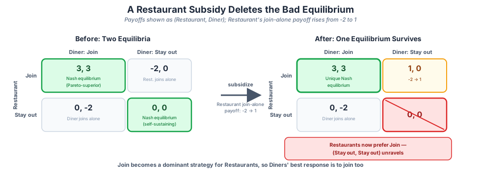
Before and after bimatrices showing a Restaurant subsidy deleting the Stay-out equilibrium — Figure 2:Raising the Restaurant’s join-alone payoff from -2 to 1 makes Join a dominant strategy for Restaurants, so Diners’ best response becomes Join too; (Stay out, Stay out) stops being a Nash equilibrium and only (Join, Join) survives.

Raising the Restaurant’s join-alone payoff from -2 to 1 makes Join a dominant strategy for Restaurants, so Diners’ best response becomes Join too; (Stay out, Stay out) stops being a Nash equilibrium and only (Join, Join) survives.

Exercise 1: Coordination without Coordination¶

Why does (Join, Join) being Pareto-superior not guarantee that it is played?
Describe the belief each side can hold at (Stay out, Stay out)
Name a real platform that may have become stuck near this bad equilibrium
What observable commitment could change one side’s best response?

Build 2: The Race to Critical Mass¶

Now suppose two platforms already have a few adopters
Platforms A and B have identical quality
Each period, one new adopter arrives
More previous adopters make a platform more attractive
This is Arthur’s increasing-returns logic in an urn-like model
Can tiny early accidents decide a large market?

A Reinforced Adoption Rule¶

Let $n_A(t)$ and $n_B(t)$ be installed bases at time $t$
The next adopter chooses A with probability

P(A \mid t) = \frac{n_A(t)^\gamma}{n_A(t)^\gamma + n_B(t)^\gamma}.

(2)

At $\gamma=1$ , this is the classic linear Pólya urn
At $\gamma>1$ , network value grows more than proportionally with installed base
We use $\gamma=2$ : identical quality, but strong increasing returns

function reinforced_adoption(T; nA0 = 1, nB0 = 1, gamma = 2.0)
    nA = nA0
    nB = nB0
    shareA = Vector{Float64}(undef, T + 1)
    shareA[1] = nA / (nA + nB)

    for t in 1:T
        weightA = nA^gamma
        weightB = nB^gamma
        if rand() < weightA / (weightA + weightB)
            nA += 1
        else
            nB += 1
        end
        shareA[t + 1] = nA / (nA + nB)
    end

    return shareA
end

reinforced_adoption (generic function with 1 method)

Random.seed!(6318)
T = 250
one_path = reinforced_adoption(T)

plot(
    0:T, one_path;
    xlabel = "New adopters",
    ylabel = "Share on Platform A",
    ylim = (0, 1),
    linewidth = 3,
    label = "A share",
    title = "One History of Two Identical Platforms",
)

Loading...

One History Is Not a Result¶

That curve feels like a story about Platform A
But A and B have exactly the same quality
Change the random seed and the story may reverse
Recall from week 6: an ABM describes a distribution over outcomes
Let us run 200 possible histories

Random.seed!(631802)
n_runs = 200
paths = reduce(hcat, [reinforced_adoption(T) for _ in 1:n_runs])
final_shares = paths[end, :]

trajectory_plot = plot(
    0:T, paths;
    color = :steelblue, alpha = 0.10, label = false,
    xlabel = "New adopters", ylabel = "Share on A", ylim = (0, 1),
    title = "200 Possible Histories",
)
final_plot = histogram(
    final_shares;
    bins = 0:0.05:1, normalize = :probability,
    color = :darkorange, alpha = 0.8, label = false,
    xlabel = "Final share on A", ylabel = "Fraction of runs",
    title = "Where the Histories End",
)

plot(trajectory_plot, final_plot; layout = (1, 2), size = (950, 360))

Loading...

lock_in_rate = mean((final_shares .<= 0.10) .| (final_shares .>= 0.90))
(lock_in_rate = lock_in_rate, A_wins = mean(final_shares .> 0.5))

(lock_in_rate = 0.98, A_wins = 0.515)

Reveal: Lock-In without a Quality Difference¶

Nearly every strongly reinforced run ends near 0 or 1
This is tipping: positive feedback pushes the market toward one dominant platform
But which platform wins is early random luck, not quality
That sensitivity to history is path dependence
Lock-in means later adopters rationally follow a lead created by earlier accidents
Important qualification: the linear case $\gamma=1$ is path dependent, but its final shares need not be winner-take-all
Winner-take-all is a result to explain, not a slogan to assume

Emergence, Again¶

As with segregation in week 6, a stark aggregate outcome emerges that no individual chose
Each adopter makes a locally sensible choice
Collectively, those choices can make one platform almost unavoidable
Sidecar entered ride-hailing early, but Uber’s growing driver-rider network helped pull later adoption toward Uber
The model does not claim quality never matters
It shows why timing and early scale can matter even when quality is equal

Exercise 2: What Breaks Lock-In?¶

Suppose users can multihome or move their data and contacts between platforms. Which change weakens lock-in more, and why?
Now give the smaller platform a clear quality advantage. How large must that gap feel before early market share stops deciding the winner?
Predict what happens to the dispersion of final market shares as the reinforcement exponent falls below 1

Build 3: Networks Matter¶

The urn treats every adopter as if they observe the whole market
Real adoption often arrives through neighbors
Recall cascades from our graph lectures
An agent adopts when enough of their neighbors have adopted
Does critical mass depend only on the number of seeds?

Random.seed!(1202)
n = 120
g_er = erdos_renyi(n, 0.05)
g_ws = watts_strogatz(n, 6, 0.08)

(
    erdos_renyi = (edges = ne(g_er), mean_degree = mean(degree(g_er))),
    watts_strogatz = (edges = ne(g_ws), mean_degree = mean(degree(g_ws))),
)

(erdos_renyi = (edges = 335, mean_degree = 5.583333333333333), watts_strogatz = (edges = 360, mean_degree = 6.0))

A Threshold Rule¶

Each node is either adopted or not adopted
Seeds adopt at time 0
Everyone else adopts when at least a fraction $\tau$ of their neighbors has adopted

a_i(t+1) = 1 \quad \text{if} \quad \frac{\sum_{j \in N(i)} a_j(t)}{|N(i)|} \ge \tau.

(3)

Updates are synchronous: everyone responds to the previous round
Adoption is irreversible in this simple model
On a small toy network with seeds $A$ and $B$ and $\tau=0.5$ : which node adopts last, and why? this figure walks through four rounds of the cascade

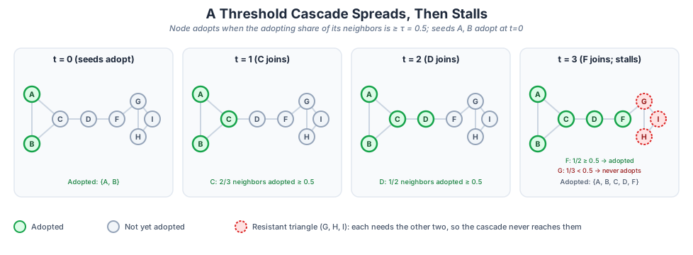
Four rounds of a threshold cascade on a small network, with a resistant triangle that never adopts — Figure 3:Seeds A and B push the cascade through C, D, and F as each crosses the τ = 0.5 threshold, but the triangle G-H-I stalls forever: G sees only 1 of its 3 neighbors adopted, and H and I see none, so none of them ever reaches τ.

Seeds A and B push the cascade through C, D, and F as each crosses the τ = 0.5 threshold, but the triangle G-H-I stalls forever: G sees only 1 of its 3 neighbors adopted, and H and I see none, so none of them ever reaches τ.

function threshold_adoption(g, seeds, tau; max_steps = 40)
    adopted = falses(nv(g))
    adopted[seeds] .= true
    adoption_rate = Float64[mean(adopted)]

    for _ in 1:max_steps
        next_adopted = copy(adopted)
        for v in vertices(g)
            if !adopted[v]
                nbrs = neighbors(g, v)
                if !isempty(nbrs) && mean(adopted[nbrs]) >= tau
                    next_adopted[v] = true
                end
            end
        end

        next_adopted == adopted && break
        adopted = next_adopted
        push!(adoption_rate, mean(adopted))
    end

    return adoption_rate
end

threshold_adoption (generic function with 1 method)

Random or Targeted Seeding?¶

We have a budget of five seeds
Strategy 1: choose five nodes at random
Strategy 2: target high-degree nodes
On the Watts-Strogatz graph, we also keep targeted seeds locally concentrated
- Local reinforcement matters when adoption uses a fractional threshold
We compare the same seed budget and the same threshold across topologies

Random.seed!(12025)
random_seeds = sort(randperm(n)[1:5])
er_degrees = degree(g_er)
ws_degrees = degree(g_ws)
er_targeted = sort(partialsortperm(er_degrees, 1:5; rev = true))

# Choose the highest-degree block of five nearby nodes on the WS ring.
ws_windows = [[mod1(start + offset, n) for offset in 0:4] for start in 1:n]
ws_targeted = ws_windows[argmax([sum(ws_degrees[w]) for w in ws_windows])]

(random = random_seeds, er_targeted = er_targeted, ws_targeted = ws_targeted)

(random = [17, 31, 32, 100, 120], er_targeted = [7, 33, 72, 80, 93], ws_targeted = [75, 76, 77, 78, 79])

tau = 0.30
curves = (
    er_random = threshold_adoption(g_er, random_seeds, tau),
    er_targeted = threshold_adoption(g_er, er_targeted, tau),
    ws_random = threshold_adoption(g_ws, random_seeds, tau),
    ws_targeted = threshold_adoption(g_ws, ws_targeted, tau),
)

p = plot(; xlabel = "Round", ylabel = "Adoption rate", ylim = (0, 1),
    title = "Five Seeds, Different Networks and Placement")
for (label, curve) in pairs(curves)
    plot!(p, 0:(length(curve) - 1), curve; marker = :circle, linewidth = 2, label = string(label))
end
p

Loading...

Reveal: Critical Mass Has a Shape¶

Five seeds are not simply five seeds
Their location determines how much local reinforcement they create
Erdős-Rényi links scatter influence differently from clustered Watts-Strogatz links
The same random seed identities can therefore produce different paths across the two graphs
Targeting high-degree nodes expands reach; concentrating seeds can help neighbors cross a fractional threshold
Tipping occurs when one round creates enough adopters to trigger the next
Topology changes where critical mass lies

A Warning about Influence¶

High degree does not automatically mean easy to persuade
A high-degree node may require many adopting neighbors to reach the same fractional threshold
Seeding a hub can be powerful because many others observe it
Waiting for a hub to adopt can be difficult because the hub observes many others
Network interventions must distinguish outgoing reach from incoming social proof
this figure contrasts the hub’s outgoing reach with the adopting neighbors it needs incoming

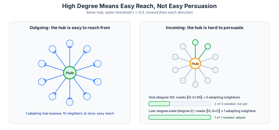
Two panels contrasting a hub's outgoing reach with the adopting neighbors it needs incoming — Figure 4:Outgoing edges show one adopting hub reaching ten neighbors at once; incoming edges show the same hub needing ⌈τ·10⌉ = 3 adopting neighbors before it adopts, versus a degree-2 node that needs only ⌈τ·2⌉ = 1. High degree amplifies reach, not persuadability.

Outgoing edges show one adopting hub reaching ten neighbors at once; incoming edges show the same hub needing ⌈τ·10⌉ = 3 adopting neighbors before it adopts, versus a degree-2 node that needs only ⌈τ·2⌉ = 1. High degree amplifies reach, not persuadability.

When Winner-Take-All Does Not Apply¶

Multihoming means participating on more than one platform
Riders can install both Uber and Lyft
Drivers can accept work from both
Multihoming weakens the feedback that makes one platform exclusive
Coexistence is more likely when switching is easy, differentiation matters, or network effects are local
Strong network effects can create concentration without creating a single winner

Craigslist and Local Network Effects¶

Craigslist looks like one giant marketplace
But a renter in Orlando gains little from apartment listings in Seattle
A job seeker may care about one occupation and one city, not the whole site
Competitors can unbundle a broad platform vertical by vertical
The relevant network effect may live inside a category, geography, or community
Before predicting winner-take-all, ask: which network is actually reinforcing which choice?

Exercise 3: Give the Better Platform an Edge¶

Let Platform A be 10% more attractive than B
Set $\theta=1.1$ and choose A with probability proportional to $\theta n_A$ versus $n_B$
Run 500 simulations
How often does the better platform finish with less than half the market?
Interpret a loss: does it prove that quality is irrelevant?

function better_platform_loss_rate(; theta = 1.1, runs = 500, T = 250)
    # TODO: repeat the adoption simulation `runs` times.
    # TODO: in each period use pA = theta * nA / (theta * nA + nB).
    # TODO: return the fraction of runs in which final nA < nB.
    return missing
end

# TODO: set a seed, call the function, and explain the result.
better_platform_loss_rate()

missing

Exercise 4: Where Do Cascades Die?¶

Use the Watts-Strogatz graph and the five targeted seeds
Vary $\tau \in \{0.1, 0.3, 0.5\}$
Plot all three adoption curves
For which thresholds does the cascade reach most of the graph?
Identify the first round in which each failed cascade stops growing

taus = [0.1, 0.3, 0.5]

# TODO: call threshold_adoption(g_ws, ws_targeted, tau) for each tau.
# TODO: plot the three curves and report where cascades die.
nothing

What We Learned¶

The chicken-and-egg problem is a coordination problem with a good and a bad equilibrium
Subsidizing one side can select the good equilibrium by changing best responses
Increasing returns can create tipping, lock-in, and path dependence
Network topology and seed placement determine whether local adoption crosses critical mass
Multihoming and local network effects limit winner-take-all predictions
We have moved from same-side and cross-side network effects to ignition
Soon we will study stable matching and the blocking pair that can unravel a proposed match

Next Time¶

Platforms must often subsidize a side to ignite
But which side, and by how much?
Is the important object the total price level or the price structure across sides?
Next time, in Platform Pricing, we make the pricing decision precise