Platform Pricing: Who Pays, Who Gets Paid

Computational Analysis of Social Complexity
Fall 2026, Spencer Lyon

Prerequisites

Outcomes

Formulate a platform’s two-sided pricing problem
Derive and solve first-order conditions numerically in Julia
Explain why optimal platform prices can be zero or negative on one side
Distinguish price structure from price level and apply the distinction to real cases

References

Required primary text: Easley & Kleinberg, Networks, Crowds, and Markets, chapter 17
Required: Rochet & Tirole, Two-Sided Markets: An Overview
Hagiu & Wright (2014)
Optional extra reading: Matchmakers (Evans & Schmalensee 2016), chapter 11

Ladies’ Night¶

A nightclub charges men $20 and women$ 0
Unfair—or is the club solving an optimization problem?
A person on either side values the club more when the other side shows up
Charging everyone the same price may leave the dance floor empty
Today we solve the platform’s actual problem and derive this asymmetry

The Pattern Is Everywhere¶

Credit cards: cardholders receive rewards while merchants pay roughly 2–3%
OpenTable: diners search and book for free while restaurants pay per seated diner
Google search: users search for free while advertisers fund the system
These are not three unrelated discounts
They are choices about who pays so that both sides participate

From Ignition to Pricing¶

In Platforms and Matchmakers we separated same-side network effects from cross-side network effects
In Ignition the chicken-and-egg problem made it hard to reach critical mass
Once participation passes a threshold, feedback can create tipping
Pricing is one lever for getting the fragile side onto the platform
First, however, we need a one-sided benchmark

using Plots
using ForwardDiff
using LaTeXStrings
using LinearAlgebra
using Random

Random.seed!(6318)
default(; linewidth=3, legend=:best, size=(760, 440))

Build 1: A One-Sided Warm-Up¶

Suppose a monopolist sells one product to one group of customers
Demand falls linearly as price rises
The firm trades off a larger margin against fewer sales
There is no second group whose participation changes customer value

Solve It by Hand¶

Let demand be $D(p)=a-bp$ and marginal cost be $c$
Profit is

\pi(p)=(p-c)(a-bp).

(1)

Differentiate only after the economic tradeoff is clear:

\pi'(p)=a+bc-2bp=0.

(2)

The interior monopoly price is

p^*=\frac{a+bc}{2b}=\frac{1}{2}\left(\frac{a}{b}+c\right).

(3)

It sits halfway between marginal cost and the choke price $a/b$

demand(p; a=10.0, b=1.0) = max(a - b * p, 0.0)
monopoly_profit(p; a=10.0, b=1.0, c=2.0) = (p - c) * demand(p; a, b)
monopoly_price(; a=10.0, b=1.0, c=2.0) = (a + b * c) / (2b)

one_sided = (a=10.0, b=1.0, c=2.0)
p_mono = monopoly_price(; one_sided...)
println("Analytic monopoly price: ", round(p_mono; digits=2))
println("Demand at the optimum: ", demand(p_mono; a=one_sided.a, b=one_sided.b))

Analytic monopoly price: 6.0


Demand at the optimum: 4.0

prices = range(0.0, one_sided.a / one_sided.b; length=301)
profits = [monopoly_profit(p; one_sided...) for p in prices]

plot(prices, profits; xlabel="price p", ylabel="profit", label=L"\pi(p)")
scatter!([p_mono], [monopoly_profit(p_mono; one_sided...)]; markersize=7, label=L"p^*=6")

Loading...

Benchmark Result¶

With $a=10$ , $b=1$ , and $c=2$ , the curve peaks at $p^*=6$
A standard one-sided monopolist with downward-sloping demand does not price below marginal cost at an interior optimum
A subsidy loses money on each sale and creates no revenue anywhere else
Keep that logic in mind—the platform result will break it

Build 2: Two Sides Must Meet¶

Now the platform serves buyers $B$ and sellers $S$
It sets per-interaction prices $p_B$ and $p_S$
One buyer without a seller creates no interaction
One seller without a buyer creates no interaction
This complementarity is the whole model

A Simplified Rochet–Tirole Model¶

Participation on each side responds to its own price:

D_B(p_B)=a_B-b_Bp_B, \qquad D_S(p_S)=a_S-b_Sp_S.

(4)

Interactions require both sides, so volume is $D_BD_S$
With cost $c$ per interaction, the margin is $p_B+p_S-c$
Profit is

\pi(p_B,p_S)=(p_B+p_S-c)D_B(p_B)D_S(p_S).

(5)

We restrict attention to prices with $D_B\geq 0$ and $D_S\geq 0$

The Cross-Side Externality¶

Raise $p_B$ and some buyers leave
A one-sided firm counts the lost buyer sales
A platform also counts the value destroyed for every seller
The same logic runs from sellers back to buyers
This is a cross-side network effect inside the profit function
Question: should the two sides still pay the same price?
this figure traces the chain in both directions

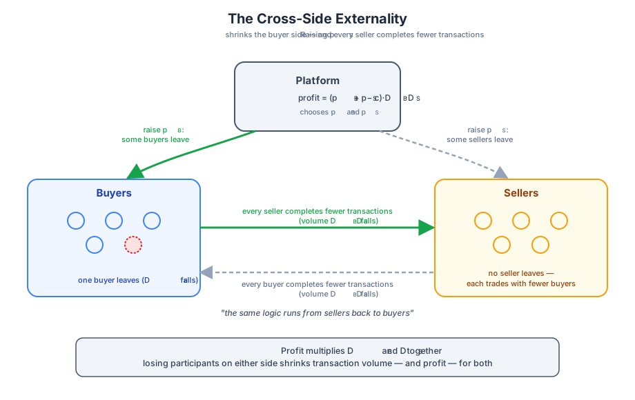
Cross-side externality loop between buyers and sellers — Figure 1:Raising $p_B$ loses buyer sales directly; because profit depends on $D_B\cdot D_S$ , fewer buyers also means every seller completes fewer transactions, even though no seller leaves. The same chain runs in reverse from a seller-price increase back to buyers.

Raising $p_B$ loses buyer sales directly; because profit depends on $D_B\cdot D_S$ , fewer buyers also means every seller completes fewer transactions, even though no seller leaves. The same chain runs in reverse from a seller-price increase back to buyers.

D_B(p_B, pars) = pars.aB - pars.bB * p_B
D_S(p_S, pars) = pars.aS - pars.bS * p_S

function platform_profit(p_B, p_S, pars)
    buyers = D_B(p_B, pars)
    sellers = D_S(p_S, pars)
    if buyers < 0 || sellers < 0
        return -Inf
    end
    return (p_B + p_S - pars.c) * buyers * sellers
end

symmetric = (aB=10.0, bB=1.0, aS=10.0, bS=1.0, c=2.0)

(aB = 10.0, bB = 1.0, aS = 10.0, bS = 1.0, c = 2.0)

Build 3: Search the Price Surface¶

Before taking derivatives, let the computer show us the landscape
We evaluate profit on a grid of feasible prices
The window includes subsidies and both choke prices
Then we mark the best grid point

pB_grid = range(-2.0, symmetric.aB / symmetric.bB; length=241)
pS_grid = range(-2.0, symmetric.aS / symmetric.bS; length=241)
profit_grid = [platform_profit(pB, pS, symmetric) for pS in pS_grid, pB in pB_grid]

grid_index = argmax(profit_grid)
grid_solution = (pB=pB_grid[grid_index[2]], pS=pS_grid[grid_index[1]])
grid_profit = profit_grid[grid_index]
println("Best grid prices: ", grid_solution)
println("Best grid profit: ", round(grid_profit; digits=2))

Best grid prices: (

pB = 4.0, pS = 4.0)
Best grid profit: 216.0

heatmap(pB_grid, pS_grid, profit_grid; xlabel=L"p_B", ylabel=L"p_S",
    color=:viridis, colorbar_title="profit", label=false)
contour!(pB_grid, pS_grid, profit_grid; levels=10, color=:white, linewidth=1, label=false)
scatter!([grid_solution.pB], [grid_solution.pS]; color=:red, markersize=8, label="grid optimum")

Loading...

What the Grid Says¶

In the symmetric case, the best grid point is $(p_B,p_S)=(4,4)$
Symmetric demand produces a symmetric price structure
A grid is transparent and robust, but only approximates the optimum
Can we recover the same answer from the first-order conditions?

Derive the First-Order Conditions¶

Write total per-interaction margin as $m=p_B+p_S-c$
For positive participation, differentiating gives

\frac{\partial \pi}{\partial p_B}=D_S[D_B-b_Bm]=0,

(6)

\frac{\partial \pi}{\partial p_S}=D_B[D_S-b_Sm]=0.

(7)

Substitute linear demand and divide by the slopes:

2p_B+p_S=\frac{a_B}{b_B}+c, \qquad p_B+2p_S=\frac{a_S}{b_S}+c.

(8)

Solving yields

p_B^*=\frac{2}{3}\frac{a_B}{b_B}-\frac{1}{3}\frac{a_S}{b_S}+\frac{c}{3},

(9)

p_S^*=\frac{2}{3}\frac{a_S}{b_S}-\frac{1}{3}\frac{a_B}{b_B}+\frac{c}{3}.

(10)

function platform_focs(x, pars)
    p_B, p_S = x
    margin = p_B + p_S - pars.c
    buyers = D_B(p_B, pars)
    sellers = D_S(p_S, pars)
    return [sellers * (buyers - pars.bB * margin),
            buyers * (sellers - pars.bS * margin)]
end

function newton_system(f, x0; tolerance=1e-10, max_iterations=50)
    x = Float64.(x0)
    for iteration in 1:max_iterations
        residual = f(x)
        if norm(residual, Inf) < tolerance
            return (root=x, iterations=iteration - 1, residual=norm(residual, Inf))
        end
        jacobian = ForwardDiff.jacobian(f, x)
        x -= jacobian \ residual
    end
    error("Newton's method did not converge")
end

newton_system (generic function with 1 method)

closed_form_prices(pars) = (
    pB=(2 * pars.aB / pars.bB - pars.aS / pars.bS + pars.c) / 3,
    pS=(2 * pars.aS / pars.bS - pars.aB / pars.bB + pars.c) / 3,
)

newton_symmetric = newton_system(x -> platform_focs(x, symmetric), [2.0, 5.0])
analytic_symmetric = closed_form_prices(symmetric)
println("Newton prices: ", round.(newton_symmetric.root; digits=6))
println("Closed-form prices: ", analytic_symmetric)
println("Distance from grid solution: ",
    norm(newton_symmetric.root - [grid_solution.pB, grid_solution.pS]))

Newton prices:

[4.0, 4.0]
Closed-form prices: (pB = 4.0, pS = 4.0)
Distance from grid solution: 0.0

Three Routes, One Answer¶

The grid search, Newton solver, and closed-form algebra all give $(4,4)$
ForwardDiff supplies the Jacobian, but the Newton updates are ours
Agreement across methods is evidence that the code matches the model
Symmetry is reassuring—but it hides the interesting economics

Break the Symmetry¶

Let buyers be much more price-sensitive than sellers
Set $b_B=4$ and $b_S=0.5$ , with both intercepts at 10 and cost at 2
Before computing: which side should the platform protect?
Losing one buyer also reduces the value delivered to sellers

asymmetric = (aB=10.0, bB=4.0, aS=10.0, bS=0.5, c=2.0)
newton_asymmetric = newton_system(x -> platform_focs(x, asymmetric), [-4.0, 13.0])
analytic_asymmetric = closed_form_prices(asymmetric)
pB_asym, pS_asym = newton_asymmetric.root

println("Buyer price: ", round(pB_asym; digits=2))
println("Seller price: ", round(pS_asym; digits=2))
println("Total price: ", round(pB_asym + pS_asym; digits=2))
println("Per-interaction margin: ", round(pB_asym + pS_asym - asymmetric.c; digits=2))
println("Closed-form check: ", analytic_asymmetric)

Buyer price: -4.33


Seller price: 13.17
Total price: 8.83
Per-interaction margin: 6.83
Closed-form check: (pB = -4.333333333333333, pS = 13.166666666666666)

Reveal 1: Subsidize the Sensitive Side¶

The optimal buyer price is about −4.33
The optimal seller price is about 13.17
The platform pays buyers to participate and charges sellers for access to them
Yet the total price is about 8.83 and the per-interaction margin is about 6.83
Ladies’ Night, cashback rewards, and free restaurant reservations fall out of the same first-order conditions
A negative price is not irrational when it creates profitable activity on the other side

Price Structure vs Price Level¶

The price level is the total charge per interaction: $p_B+p_S$
The price structure is how that total is divided between the two sides
Holding $p_B+p_S$ fixed but changing the split changes participation and volume
That would be impossible in a genuinely one-sided market
This sensitivity to price structure is Rochet and Tirole’s key definition of two-sidedness

Reveal 2: Comparative Statics¶

One asymmetric example could be a coincidence
Sweep buyer price sensitivity $b_B$ while holding the seller side fixed
Trace both optimal prices and find the zero-price crossover
Prediction: as buyers become easier to lose, buyers pay less and sellers pay more

buyer_slopes = range(0.4, 6.0; length=240)
sweep_parameters = [merge(asymmetric, (bB=b,)) for b in buyer_slopes]
sweep_prices = closed_form_prices.(sweep_parameters)
buyer_prices = getproperty.(sweep_prices, :pB)
seller_prices = getproperty.(sweep_prices, :pS)
zero_crossover = 2 * asymmetric.aB / (asymmetric.aS / asymmetric.bS - asymmetric.c)

plot(buyer_slopes, buyer_prices; xlabel=L"b_B", ylabel="optimal price", label=L"p_B^*")
plot!(buyer_slopes, seller_prices; label=L"p_S^*")
hline!([0.0]; color=:black, linestyle=:dot, linewidth=1.5, label="zero price")
vline!([zero_crossover]; color=:gray, linestyle=:dash, linewidth=2,
    label="crossover ≈ $(round(zero_crossover; digits=2))")

Loading...

Reading the Sweep¶

The buyer price crosses zero at $b_B\approx 1.11$ for these parameters
Beyond that point, greater buyer sensitivity produces a larger buyer subsidy
The seller price rises because sellers benefit from the participation that subsidy creates
A one-sided monopolist would NEVER price below cost; a platform does it routinely and rationally
The qualification matters: the platform earns revenue from the cross-side response

Pricing Can Help a Platform Ignite¶

Subsidizing one side can help solve the chicken-and-egg problem
Reaching critical mass strengthens cross-side participation and may trigger tipping
Same-side congestion or rivalry can push in the opposite direction
Our static linear model compresses those dynamics into demand curves
The lesson is not “always subsidize buyers”; it is “price the network effect, not just the transaction”

Platforms in Court¶

Ohio v. American Express treated credit-card transactions as a two-sided platform market
- Evaluating merchant fees alone can miss cardholder rewards and changes in transaction volume
Epic Games v. Apple put platform market definition and rules between users and developers at center stage
- A developer commission cannot be interpreted without asking how users and developers respond together
Courts increasingly require two-sided analysis when the relevant market links both groups
Two-sided analysis does not mean every platform practice is efficient or lawful

Multihoming and the Competitive Bottleneck¶

Multihoming means participating on more than one platform
Armstrong’s competitive-bottleneck insight in one line:
- Platforms court the side that single-homes and tax the side that multihomes
the diagram below shows why: access to the single-homers is what rival platforms compete over
Winning a single-homing participant can give access to that participant across competing platforms
This adds competitive strategy to the cross-side logic in our monopoly model

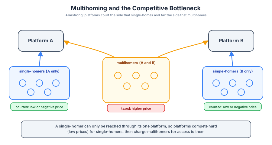
Competitive bottleneck: single-homers courted, multihomers taxed — Figure 2:Single-homing users are split between rival platforms and courted with low or negative prices, while multihoming users connect to both platforms and are taxed with higher prices, because access to the single-homers is what the platforms are really competing for.

Single-homing users are split between rival platforms and courted with low or negative prices, while multihoming users connect to both platforms and are taxed with higher prices, because access to the single-homers is what the platforms are really competing for.

Exercise 1: Platform or Tariff?¶

Consider Costco membership, Amazon Prime, and a farmers-market stall fee
Is each example two-sided pricing or a plain two-part tariff?
Identify the sides and the cross-side interaction, if any
Use the test: would changing the price structure while holding the price level fixed change volume?
Be ready to defend why a label such as “membership” or “fee” is not enough

Exercise 2: More Sellers¶

Return to the asymmetric parameterization
Double the seller intercept from $a_S=10$ to $a_S=20$
Re-solve for $p_B^*$ and $p_S^*$
Which price rises? Which falls?
Explain the result using the value of attracting the opposite side—not algebra alone

more_sellers = merge(asymmetric, (aS=20.0,))

# TODO: compute the new optimum with closed_form_prices or newton_system
# TODO: compare both prices with analytic_asymmetric
# TODO: explain why the changes have opposite signs

(aB = 10.0, bB = 4.0, aS = 20.0, bS = 0.5, c = 2.0)

Exercise 3: Charge for Membership Instead¶

Our model charges each side per interaction
Consider membership fees $F_B$ and $F_S$ , each paid once
With per-interaction cost $c$ , profit becomes

\pi_M(F_B,F_S)=F_BD_B(F_B)+F_SD_S(F_S)-cD_B(F_B)D_S(F_S).

(11)

Find the best membership fees on the grid
Compare fees, participation, interaction volume, and profit with the usage-fee optimum
Why are dollar values not directly interchangeable across the two models?

function membership_profit(F_B, F_S, pars)
    buyers = D_B(F_B, pars)
    sellers = D_S(F_S, pars)
    if buyers < 0 || sellers < 0
        return -Inf
    end
    return F_B * buyers + F_S * sellers - pars.c * buyers * sellers
end

membership_B_grid = range(-5.0, asymmetric.aB / asymmetric.bB; length=301)
membership_S_grid = range(-5.0, asymmetric.aS / asymmetric.bS; length=301)

# TODO: evaluate membership_profit over both grids
# TODO: locate the maximizing pair of membership fees
# TODO: compare participation, volume, and profit across pricing models

-5.0:0.08333333333333333:20.0

Exercise 4: Design a Compute Marketplace¶

You run a GPU-compute marketplace matching AI startups to datacenter owners
This previews our AI agents unit: startups deploy agents but need scarce compute
Which side would you subsidize at launch, and why?
Discuss price sensitivity, cross-side value, the chicken-and-egg problem, and multihoming
What evidence would make you reverse the subsidy?
Design one non-price incentive that could help reach critical mass

Takeaways¶

A platform chooses a vector of prices, not one price
Cross-side network effects make participation on each side affect the value of the other
The price-sensitive side may optimally pay zero or receive a subsidy
Price structure can change volume even when the total price level does not
Grid search, hand-derived first-order conditions, and Newton’s method tell the same story
As with Braess' paradox, familiar pieces can produce a surprising system-level result

Next Time: Markets Without Prices¶

Prices are one way to clear a market—but some markets refuse prices entirely
Kidneys. Medical residencies. School seats.
These markets match instead of price
We will define a stable matching and ask whether any blocking pair can upset it
Then we will build the deferred-acceptance algorithm that helped win a Nobel